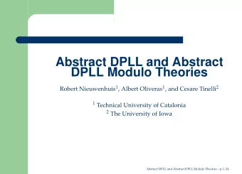
DPLL( T ):Fast Decision Procedures Harald Ganzinger George Hagen - PowerPoint PPT Presentation

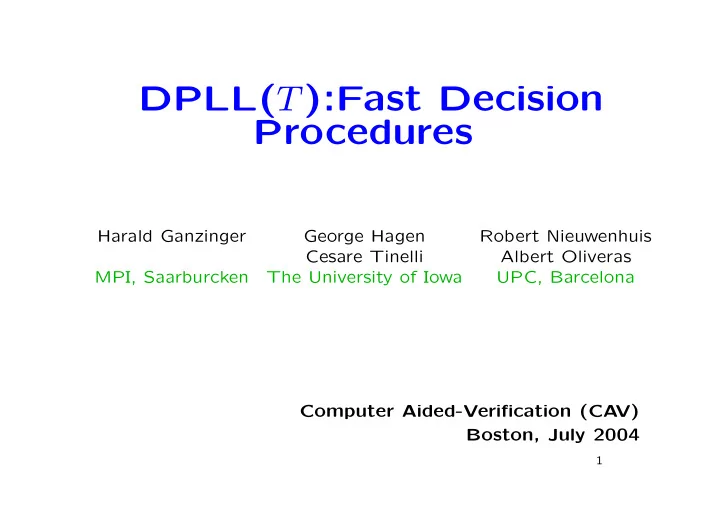
DPLL( T ):Fast Decision Procedures Harald Ganzinger George Hagen Robert Nieuwenhuis Cesare Tinelli Albert Oliveras MPI, Saarburcken The University of Iowa UPC, Barcelona Computer Aided-Verification (CA V) Boston, July 2004 1

In Memoriam Harald Ganzinger (1950-2004) 2

Overview of this talk 1. Introduction 2. Lazy vs eager approach Lazy approach: advantages and disadvantages Eager approach: advantages and disadvantages 3. DPLL( T ): Our framework for SMT The DPLL algorithm Branching heuristics, unit propagation and conflict analysis Comparison with existing approaches 4. A concrete case: EUF with offsets A solver for EUF Experimental results 5. Conclusions and future work 3

1.-Introduction SMT: Satisfiability modulo theories g ( a )= c ∧ ( f ( g ( a )) � = f ( c ) ∨ g ( a )= d ) ∧ c � = d Theories of interest: EUF [Burch and Dill ’94], CLU [Bryant, Lahiri and Seshia ’02], separation logic [BLS ’03], arrays, ... Applications: circuit design, compiler optimization, planning, scheduling, software/hardware verification, ... 4

2.-State of the art Lazy vs eager approach Lazy approach The following three steps are iterated SAT solver looks for a propositional model Specialized procedure for conjunctions of literals checks its consistency If model consistent then formula is SAT, otherwise a lemma is added precluding the model – constraints imposed by the theory introduced on demand – Lazy/eager notification, online/offline SAT solver, extraction of inconsistency proofs [Armando et al ’00; deMoura and Ruess ’02; Barret, Dill and Stump ’02; Flanagan et al ’03, etc] 5

2.-Lazy vs eager approach Lazy vs eager approach Lazy approach Advantages: • Use of off-the-shelf theory solvers • Can use of almost off-the-shelf SAT solvers Disadvantages: • Information from the theory only used to validate propositional models • Too many iterations may be required Tools: SVC, CVC (Lite), ICS, VeriFun, MathSAT 6

2.-Lazy vs eager approach Lazy vs eager approach Eager approach formula converted into an equisatisfiable propositional one to be checked by a SAT solver Two steps (for CLU) • Functional symbols are removed, only constants left • (in)Equality is removed Small-domain encoding (SD) [Pnuelli et al ’99, BLS ’02], Per-constraint encoding (EIJ) [Bryant, German and Velev ’02; Bryant and Velev ’02], Hybrid methods [BLS ’02, ’03] 7

2.-State of the art Lazy vs eager approach Eager approach: different encodings Given the equality formula: ( k 1 = k 2 ∨ k 3 = k 4 ) ( k 2 = k 3 ∨ k 1 = k 4 ∨ k 2 = k 4 ) ∧ Small Domain encoding (SD): propositional formula small but suffers from loss of structure ( x 11 ∨ (( x 31 ∧ x 41 ) ∨ ( ¬ x 31 ∧ x 32 ∧ ¬ x 41 )) ) ∧ ( x 31 ∨ (( x 11 ∧ x 41 ) ∨ ( ¬ x 11 ∧ x 12 ∧ ¬ x 41 )) ∨ x 41 ) Per-constraing encoding (EIJ): structure preserved but size may be exponential if pred/succ allowed ( e 12 ∨ e 34 ) ∧ ( e 23 ∨ e 14 ∨ e 24 ) e 12 ∧ e 24 ⇒ e 14 e 12 ∧ e 14 ⇒ e 24 . . . 8

2.-Lazy vs eager approach Lazy vs eager approach Eager approach Advantages: • Best SAT solver may be used as is • Theory information compiled into the translated formula Disadvantages: • Loss of formula structure, exponential blowup in size • Limited range of application Tools: UCLID 9

3.-DPLL( T ): Our framework for SMT Our framework for SMT DPLL(X) Solver T ❅ � ❅ � ❅ � ❅ � ❅ � ❅ � ❅ � ❅ � ❅ � ❅ � ❅ � ❅ � ❅ � ❅ � ❘ ❅ � ✠ DPLL(T) Based on theoretical calculus in [Tinelli’02] 10

3.-DPLL( T ): Our framework for SMT Our framework for SMT Solver T ✬ ✩ Set a = b to true DPLL(X) ✲ ❅ a = b ❅ ❅ ✫ ✪ ❅ ✟ ❅ ✟ ✟ ❅ ✟ ✟ ❅ ✟ ✟ ❅ ✟ ✟ ❅ ✟ ✟ ❅ ✟ ✟ ❅ ✟ ✟ ❅ ✟ ✟ ❅ ✟ ✟ ❅ ✟ ✙ ❅ ❘ DPLL(T) 11

3.-DPLL( T ): Our framework for SMT Our framework for SMT Solver T ✬ ✩ DPLL(X) ✛ f ( a )= f ( b ) Consequences: a = b ❅ a = b g ( a )= g ( b ) f ( a )= f ( b ) ❅ ❅ ✫ ✪ ❅ g ( a )= g ( b ) ✟ ❅ ✟ ✟ ❅ ✟ ✟ ❅ ✟ ✟ ❅ ✟ ✟ ❅ ✟ ✟ ❅ ✟ ✟ ❅ ✟ ✟ ❅ ✟ ✟ ❅ ✟ ✟ ❅ ✟ ✙ ❘ ❅ DPLL(T) 12

3.-DPLL( T ): Our framework for SMT Our framework for SMT Solver T ✬ ✩ Set f ( c ) � = e to true DPLL(X) ✲ f ( c ) � = e f ( a )= f ( b ) ❅ a = b g ( a )= g ( b ) ❅ ❅ ✫ ✪ ❅ ✟ ❅ ✟ ✟ ❅ ✟ ✟ ❅ ✟ ✟ ❅ ✟ ✟ ❅ ✟ ✟ ❅ ✟ ✟ ❅ ✟ ✟ ❅ ✟ ✟ ❅ ✟ ✟ ❅ ✙ ✟ ❅ ❘ DPLL(T) 13

3.-DPLL( T ): Our framework for SMT Our framework for SMT Solver T ✬ ✩ DPLL(X) ✛ f ( c ) � = e f ( a )= f ( b ) Consequences: f ( c ) � = e ❅ a = b g ( a )= g ( b ) ❅ ❅ ✫ ✪ ❅ ✟ ❅ ✟ ✟ ❅ ✟ ✟ ❅ ✟ ✟ ❅ ✟ ✟ ❅ ✟ ✟ ❅ ✟ ✟ ❅ ✟ ✟ ❅ ✟ ✟ ❅ ✟ ✟ ❅ ✙ ✟ ❅ ❘ DPLL(T) 14

3.-DPLL( T ): Our framework for SMT Our framework for SMT Solver T ✬ ✩ Set c = a to true c = a DPLL(X) ✲ f ( c ) � = e f ( a )= f ( b ) ❅ a = b g ( a )= g ( b ) ❅ ❅ ✫ ✪ ❅ ✟ ❅ ✟ ✟ ❅ ✟ ✟ ❅ ✟ ✟ ❅ ✟ ✟ ❅ ✟ ✟ ❅ ✟ ✟ ❅ ✟ ✟ ❅ ✟ ✟ ❅ ✟ ✟ ❅ ✟ ✙ ❘ ❅ DPLL(T) 15

3.-DPLL( T ): Our framework for SMT Our framework for SMT Solver T ✬ ✩ f ( b ) � = e c = a f ( a ) � = e DPLL(X) ✛ f ( c ) � = e f ( a )= f ( b ) Consequences: c = a ❅ a = b g ( a )= g ( b ) f ( a ) � = e ❅ ❅ ✫ ✪ ❅ f ( b ) � = e ✟ ❅ ✟ ✟ ❅ ✟ ✟ ❅ ✟ ✟ ❅ ✟ ✟ ❅ ✟ ✟ ❅ ✟ ✟ ❅ ✟ ✟ ❅ ✟ ✟ ❅ ✟ ✟ ❅ ✟ ✙ ❅ ❘ DPLL(T) 16

3.-DPLL( T ): Our framework for SMT Our framework for SMT Solver T ✬ ✩ f ( b ) � = e Is f ( a )= f ( b ) true ? c = a f ( a ) � = e DPLL(X) ✲ f ( c ) � = e f ( a )= f ( b ) ❅ a = b g ( a )= g ( b ) ❅ ❅ ✫ ✪ ❅ ✟ ❅ ✟ ✟ ❅ ✟ ✟ ❅ ✟ ✟ ❅ ✟ ✟ ❅ ✟ ✟ ❅ ✟ ✟ ❅ ✟ ✟ ❅ ✟ ✟ ❅ ✟ ✟ ❅ ✙ ✟ ❅ ❘ DPLL(T) 17

3.-DPLL( T ): Our framework for SMT Our framework for SMT Solver T ✬ ✩ f ( b ) � = e c = a f ( a ) � = e DPLL(X) ✛ f ( c ) � = e f ( a )= f ( b ) YES ❅ a = b g ( a )= g ( b ) ❅ ❅ ✫ ✪ ❅ ✟ ❅ ✟ ✟ ❅ ✟ ✟ ❅ ✟ ✟ ❅ ✟ ✟ ❅ ✟ ✟ ❅ ✟ ✟ ❅ ✟ ✟ ❅ ✟ ✟ ❅ ✟ ✟ ❅ ✙ ✟ ❅ ❘ DPLL(T) 18

3.-DPLL( T ): Our framework for SMT Our framework for SMT Solver T ✬ ✩ f ( b ) � = e Why is f ( a ) � = e true? c = a f ( a ) � = e DPLL(X) ✲ f ( c ) � = e f ( a )= f ( b ) ❅ a = b g ( a )= g ( b ) ❅ ❅ ✫ ✪ ❅ ✟ ❅ ✟ ✟ ❅ ✟ ✟ ❅ ✟ ✟ ❅ ✟ ✟ ❅ ✟ ✟ ❅ ✟ ✟ ❅ ✟ ✟ ❅ ✟ ✟ ❅ ✟ ✟ ❅ ✙ ✟ ❅ ❘ DPLL(T) 19

3.-DPLL( T ): Our framework for SMT Our framework for SMT Solver T ✬ ✩ f ( b ) � = e c = a f ( a ) � = e DPLL(X) ✛ f ( c ) � = e f ( a )= f ( b ) Because c = a , f ( c ) � = e ❅ a = b g ( a )= g ( b ) ❅ ❅ ✫ ✪ ❅ ✟ ❅ ✟ ✟ ❅ ✟ ✟ ❅ ✟ ✟ ❅ ✟ ✟ ❅ ✟ ✟ ❅ ✟ ✟ ❅ ✟ ✟ ❅ ✟ ✟ ❅ ✟ ✟ ❅ ✙ ✟ ❅ ❘ DPLL(T) 20

3.-DPLL( T ): Our framework for SMT Our framework for SMT Solver T ✬ ✩ f ( b ) � = e Backtrack 2 steps c = a f ( a ) � = e DPLL(X) ✲ f ( c ) � = e f ( a )= f ( b ) ❅ a = b g ( a )= g ( b ) ❅ ❅ ✫ ✪ ❅ ✟ ❅ ✟ ✟ ❅ ✟ ✟ ❅ ✟ ✟ ❅ ✟ ✟ ❅ ✟ ✟ ❅ ✟ ✟ ❅ ✟ ✟ ❅ ✟ ✟ ❅ ✟ ✟ ❅ ✙ ✟ ❅ ❘ DPLL(T) 21

3.-DPLL( T ): Our framework for SMT Our framework for SMT Solver T ✬ ✩ DPLL(X) ✛ f ( a )= f ( b ) ❅ a = b g ( a )= g ( b ) ❅ ❅ ✫ ✪ ❅ ✟ ❅ ✟ ✟ ❅ ✟ ✟ ❅ ✟ ✟ ❅ ✟ ✟ ❅ ✟ ✟ ❅ ✟ ✟ ❅ ✟ ✟ ❅ ✟ ✟ ❅ ✟ ✟ ❅ ✟ ✙ ❘ ❅ DPLL(T) 22

3.-DPLL( T ): Our framework for SMT The Davis-Putnam algorithm (DPLL) Depth-first search algorithm with backtracking At each point, the algorithm keeps a partial interpretation and tries to extend it Three successful mechanisms to speed up the search • Branching heuristic: determines the literal to extend the interpretation • Unit propagation: prunes the search space • Conflict Analysis: indicates where to backtrack to and adds lemmas 23

3.-DPLL( T ): Our framework for SMT Branching heuristics Unassigned literal with the highest score is selected New literals introduced in CNF translation can be selected VSIDS heuristic [Moskewicz et al ’01] 24

3.-DPLL( T ): Our framework for SMT T-based Branching heuristics Unassigned literal with the highest score is selected New literals introduced in CNF translation can be selected VSIDS heuristic [Moskewicz et al ’01] Theory-dependent heuristics 25