Distributional Results for Thresholding Estimators in - PowerPoint PPT Presentation

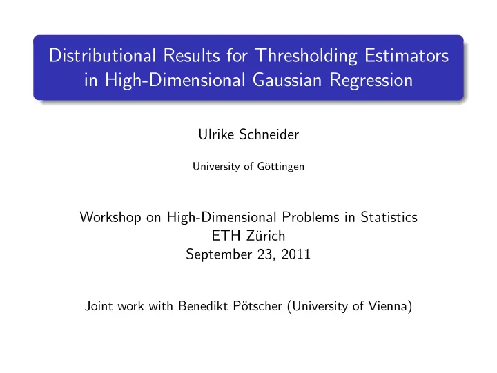
Distributional Results for Thresholding Estimators in High-Dimensional Gaussian Regression Ulrike Schneider University of G¨ ottingen Workshop on High-Dimensional Problems in Statistics ETH Z¨ urich September 23, 2011 Joint work with Benedikt P¨ otscher (University of Vienna)

Penalized LS (ML) Estimators Linear regression model y = θ 1 x . 1 + . . . θ k x . k + ε = X θ + ε response y ∈ R n regressors x . i ∈ R n , 1 ≤ i ≤ k errors ε ∈ R n parameter vector θ = ( θ 1 , . . . , θ k ) ′ ∈ R k A penalized least-squares (PLSE) or maximum-likelihood estimator (PMLE) ˆ θ for θ is given by ˆ � y − X θ � 2 θ = arg min + P n ( θ ) , θ ∈ R k � �� � � �� � likelihood or LS -part penalty where X = [ x . 1 , . . . , x . k ] is the n × k regressor matrix. 1 / 1

Penalized LS (ML) Estimators (cont’d) General class of Bridge-estimators (Frank & Friedman, 1993) k � | θ i | γ P n ( θ ) = λ n i =1 Ridge-estimator (Hoerl & Kennard, 1970) γ = 2: Lasso (Tibshirani, 1996). γ = 1: Hard- and soft-thresholding estimators. SCAD estimator (Fan & Li, 2001) Elastic-net estimator (Zou & Hastie, 2005) Adaptive Lasso estimator (Zou, 2006) (thresholded) Lasso with refitting (Van de Geer et al, 2010; Belloni & Chernozhukov, 2011) MCP (Zhang, 2010) . . . 2 / 1

Relationship to classical PMS-estimators Brigde-estimators satisfy k � θ ∈ R k � y − X θ � 2 + λ n | θ i | γ min (0 < γ < ∞ ) i =1 For γ → 0, get θ ∈ R k � y − X θ � 2 + λ n card { i : θ i � = 0 } min which yields a minimum C p -type procedure such as AIC and BIC. ( l γ -type penalty with “ γ = 0”) → ‘classical’ post-modelselection (PMS) estimators. 3 / 1

Relationship to classical PMS-estimators (cont’d) For “ γ = 0” procedures are computationally expensive. For γ > 0 (Bridge) estimators are more computationally tractable, especially for γ ≥ 1 (convex objective function). For γ ≤ 1, estimators perform model selection P (ˆ θ i = 0) > 0 if θ i = 0 . Phenomenon is more pronounced for smaller γ . γ = 1 (Lasso and adaptive Lasso) as compromise between the wish to detect zeros and computational simplicity. The PLSEs (and thresholding estimators) we treat in the following can be viewed to simultaneously perform model selection and parameter estimation. 4 / 1

Some terminology Consistent model selection n →∞ P (ˆ lim θ i = 0) = 1 whenever θ i = 0 (1 ≤ i ≤ k ) Estimator is sparse or sparsely tuned. Conservative model selection n →∞ P (ˆ lim θ i = 0) < 1 whenever θ i = 0 (1 ≤ i ≤ k ) Estimator is non-sparsely tuned. Consistent vs. conservative model selection can in our context be driven by the (asymptotic) behavior of the tuning parameter. 5 / 1

Literature on distributional properties of PLSEs - fixed-parameter asymptotic framework (non-uniformity issues) - sparsely-tuned PLSEs Oracle property – obtain same asymptotic distribution as ‘oracle estimator’ (infeasible unpenalized estimator using the true zero restrictions). Fan & Li, 2001. (SCAD) Zou, 2006. (Lasso and adaptive Lasso) Cai, Fan, Li & Zhou (2002), Fan & Li (2002, 2004), Bunea (2004), Fan & Peng (2006), Bunea & McKeague (2005), Hunter & Li (2005), Fan, Li & Zhou (2006), Wang & Leng (2007), Wang, G. Li, & Tsai (2007), Zhang & Lu (2007), Wang, R. Li, & Tsai (2007), Huang, Horowitz & Ma (2008), Li & Liang (2008), Zou & Yuan (2008), Zou & Li (2008), Johnson, Lin, & Zeng (2008), Zou & Li (2008), Zou & Yuan (2008), Lin, Xiang & Zhang (2009), Xie & Huang (2009), Zhu & Zhu (2009), Zou & Zhang (2009) . . . 6 / 1

Literature on distributional properties of PLSEs (cont’d) - moving-parameter asymptotic framework (taking non-uniformity into account) - Sparsely and non-sparsely tuned PLSEs. Knight & Fu, 2000. (Non-sparsely tuned Lasso and Bridge estimators for q < 1 in general.) P¨ otscher & Leeb (2009), P¨ otscher & S., (2009), P¨ otscher & S. (2010), P¨ otscher & S. (2011). 7 / 1

Assumptions and Notation y = X θ + ε X is non-stochastic ( n × k ), rk ( X ) = k ( ⇒ k ≤ n ). No further assumptions on X . k may vary with n . ε ∼ N n (0 , σ 2 I n ) � ( X ′ X / n ) − 1 � Notation: ξ 2 i , n := ( X ′ X = n I k ⇒ ξ i,n = 1) i , i ˆ θ LS = ( X ′ X ) − 1 X ′ y LS = � y − X ˆ σ 2 θ LS � 2 / ( n − k ) ˆ Consider 3 estimators: hard-, soft- and adaptive soft-thresholding acting componentwise. 8 / 1

Hard-thresholding ˜ θ H , i θ H , i = ˆ ˜ θ LS , i 1 ( | ˆ θ LS , i | > ˆ σ LS ξ i,n η i,n ) 9 / 1

Hard-thresholding ˜ θ H , i θ H , i = ˆ ˜ θ LS , i 1 ( | ˆ θ LS , i | > ˆ σ LS ξ i,n η i,n ) orthogonal case: equivalent to a pretest estimator based on t-tests or C p crite- rion such as AIC, BIC (classical post-model selection estima- tor) with penalty term � � P n ( θ ) = � k σ LS ξ i,n η i,n ) 2 − ( | θ i | − ˆ σ LS ξ i,n η i,n ) 2 1 ( | θ i | < ˆ (ˆ σ LS ξ i,n η i,n ) i =1 n also equivalent to MCP 9 / 1

Soft-thresholding ˜ θ S , i θ S , i = sign(ˆ ˜ θ LS , i ) ( | ˆ θ LS , i | − ˆ σ LS ξ i,n η i,n ) + 10 / 1

Soft-thresholding ˜ θ S , i θ S , i = sign(ˆ ˜ θ LS , i ) ( | ˆ θ LS , i | − ˆ σ LS ξ i,n η i,n ) + orthogonal case: equivalent to Lasso with penalty term � k P n ( θ ) = 2 n ˆ σ LS i =1 ξ i,n η i,n | θ i | also equivalent to Dantzig selector 10 / 1

Adaptive soft-thresholding ˜ θ AS , i � if | ˆ 0 θ LS , i | ≤ ˆ σ LS ξ i,n η i,n ˜ θ AS , i = ˆ σ LS ξ i,n η i,n ) 2 / ˆ if | ˆ θ LS , i − (ˆ θ LS , i θ LS , i | > ˆ σ LS ξ i,n η i,n 11 / 1

Adaptive soft-thresholding ˜ θ AS , i � if | ˆ 0 θ LS , i | ≤ ˆ σ LS ξ i,n η i,n ˜ θ AS , i = ˆ σ LS ξ i,n η i,n ) 2 / ˆ if | ˆ θ LS , i − (ˆ θ LS , i θ LS , i | > ˆ σ LS ξ i,n η i,n orthogonal case: equivalent to adaptive Lasso with penalty term � k i =1 ( ξ i,n η i,n ) 2 | θ i | / | ˆ σ 2 P n ( θ ) = 2 n ˆ θ LS , i | LS also equivalent to non-negative Garotte (Breiman, 1995) 11 / 1

“Infeasible” versions Known-variance case: θ H , i = ˆ ˆ θ LS , i 1 ( | ˆ θ LS , i | > σξ i,n η i,n ) θ S , i = sign(ˆ ˆ θ LS , i ) ( | ˆ θ LS , i | − σξ i,n η i,n ) + � if | ˆ 0 θ LS , i | ≤ σξ i,n η i,n ˆ θ AS , i = θ LS , i − ( σξ i,n η i,n ) 2 / ˆ ˆ if | ˆ θ LS , i θ LS , i | > σξ i,n η i,n 12 / 1

Variable selection We shall assume that sup ξ i,n / n 1 / 2 < ∞ . Let ˇ θ i stand for any of the estimators ˆ θ H , i , ˆ θ S , i , ˆ θ AS , i , ˜ θ H , i , ˜ θ S , i , ˜ θ AS , i . Variable selection P n ,θ,σ (ˇ θ i = 0) → 0 for any θ with θ i � = 0 ⇐ ⇒ ξ i,n η i,n → 0 P n ,θ,σ (ˇ ⇒ n 1 / 2 η i,n → ∞ θ i = 0) → 1 for any θ with θ i = 0 ⇐ P n ,θ,σ (ˇ ⇒ n 1 / 2 η i,n → e i θ i = 0) → c i < 1 for any θ with θ i = 0 ⇐ with 0 ≤ e i < ∞ 1 ( ξ i,n η i,n → 0 and) n 1 / 2 η i,n → e i < ∞ leads to (sensible) conserva- tive selection. 2 ( ξ i,n η i,n → 0 and) n 1 / 2 η i,n → ∞ leads to (sensible) consistent selection. 13 / 1

Parameter estimation, minimax rate Consistency ⇒ ξ i,n η i,n → 0 and ξ i,n / n 1 / 2 → 0 ˇ θ i is consistent for θ i ⇐ Suppose ξ i,n η i,n → 0 and ξ i,n / n 1 / 2 → 0 . Then ˇ θ i is uniformly consistent for θ i in the sense that for all ε > 0 there exists a real number M > 0 such that P n ,θ,σ ( | ˇ sup sup sup θ i − θ i | > σ M ) < ε 0 <σ< ∞ n ∈ N θ ∈ R k Suppose ξ i,n η i,n → 0 , ξ i,n / n 1 / 2 → 0 , and b i , n ≥ 0 . If for all ε > 0 there exists a real number M > 0 such that P n ,θ,σ ( b i,n | ˇ sup sup sup θ i − θ i | > σ M ) < ε. n ∈ N θ ∈ R k 0 <σ< ∞ Then b i,n = O ( a i,n ) , where a i,n = min( n 1 / 2 /ξ i,n , ( ξ i,n η i,n ) − 1 ) 14 / 1

Parameter estimation, minimax rate (cont’d) Minimax rate is ξ i,n / n 1 / 2 in the conservative case, and 1 2 only ξ i,n η i,n = o ( ξ i,n / n 1 / 2 ) in the consistent case. 15 / 1

Finite sample distribution: hard-thresholding ˆ θ H , i H , n ,θ,σ ( x ) = P n ,θ,σ ( α i,n /σ (ˆ F i θ H , i − θ i ) ≤ x ) (known-variance case) dF i H , n ,θ,σ ( x ) = � � Φ( n 1 / 2 ( − θ i / ( σξ i,n ) + η i,n )) − Φ( n 1 / 2 ( − θ i / ( σξ i,n ) − η i,n )) d δ − α i,n θ i /σ ( x ) + n 1 / 2 / ( α i,n ξ i,n ) φ ( n 1 / 2 x / ( α i,n ξ i,n )) 1 ( | α − 1 i,n x + θ i /σ | > ξ i,n η i,n ) dx , where φ and Φ are the pdf and cdf of N (0 , 1), resp. 16 / 1

Finite sample distribution: hard-thresholding ˆ θ H , i n = 40 , η i,n = 0 . 05 , θ i = 0 . 16 , ξ i,n = 1 , σ = 1 , α i,n = n 1 / 2 /ξ i,n 16 / 1

Finite sample distribution: hard-thresholding ˜ θ H , i ˜ H , n ,θ,σ ( x ) = P n ,θ,σ ( α i,n /σ (˜ F i θ H , i − θ i ) ≤ x ) (unknown-variance case) d ˜ F i H , n ,θ,σ ( x ) = � ∞ { Φ( n 1 / 2 ( − θ i / ( σξ i,n ) + s η i,n ) − Φ( n 1 / 2 ( − θ i / ( σξ i,n ) − s η i,n ) } ρ n − k ( s ) ds d δ − α i,n θ i /σ ( x ) 0 � ∞ + n 1 / 2 α − 1 i,n ξ − 1 i,n φ ( n 1 / 2 x / ( α i,n ξ i,n )) 1 ( | α − 1 i,n x + θ i /σ | > ξ i,n s η i,n ) ρ n − k ( s ) ds dx , 0 � χ 2 n − k / ( n − k ) . where ρ n − k is the density of 17 / 1