Discretization and Symmetry Rob F. Remis and J orn T. Zimmerling - PowerPoint PPT Presentation
Discretization and Symmetry Rob F. Remis and J orn T. Zimmerling DCSE Fall School, Delft, November 4 8, 2019 1 Introduction Objective Discretize Maxwells equation to formulate model order reduction using linear algebra Symmetry in
Discretization and Symmetry Rob F. Remis and J¨ orn T. Zimmerling DCSE Fall School, Delft, November 4 – 8, 2019 1
Introduction Objective Discretize Maxwell’s equation to formulate model order reduction using linear algebra Symmetry in the discrete domain Application of this theory to imaging 2
Instantaneously Reacting Material: 1D One-dimensional Maxwell equation �� 0 � � σ � � ε � � � E z � � J ext � 0 0 ∂ y z + + = − (1) ∂ t , ∂ y 0 0 0 0 µ H y 0 succinctly written as [ D + S + M ∂ t ] f = − q , (2) Discretization: differential operators & functions �→ matrices and vectors 3
Maxwell on a grid E z ( y 0 ) E z ( y 1 ) E z ( y 2 ) E z ( y 3 ) E z ( y Q ) E z ( y Q +1 ) δ Q +1 δ 1 δ 2 δ 3 ˆ ˆ ˆ y = 0 y = L δ 1 δ 2 δ n H x (ˆ y 1 ) H x (ˆ y 2 ) H x (ˆ y 3 ) H x (ˆ y Q ) H x (ˆ y Q +1 ) 4
Maxwell on a grid E z ( y Q ) E z ( y Q +1 ) E z ( y 0 ) E z ( y 1 ) E z ( y 2 ) E z ( y 3 ) δ Q +1 δ 1 δ 2 δ 3 ˆ ˆ ˆ y = 0 y = L δ 1 δ 2 δ n H x (ˆ y 1 ) H x (ˆ y 2 ) H x (ˆ y 3 ) H x (ˆ y Q ) H x (ˆ y Q +1 ) We discretize the equation ∂ y H x | y = y q + σ ( y q ) E z ( y q , t ) ε r ( y q ) ∂ t E z ( y q , t ) = −J ext ( y q , t ) , z on primary grid for q = 1 , 2 , ..., Q and ∂ y E z | y =ˆ y q + µ (ˆ y q ) ∂ t H x (ˆ y q , t ) = 0 on the dual grid for q = 1 , 2 , ..., Q + 1. 5
Discrete Equations We finally arrive at h x (ˆ y q +1 , t ) − h x (ˆ y q , t ) + σ ( y q ) e z ( y q , t ) + ε ( y q ) ∂ t e z ( y q , t ) = − j ext ( y q , t ) , z ˆ δ y ; q for q = 1 , 2 , ..., Q and e z ( y q , t ) − e z ( y q − 1 , t ) + µ (ˆ y q ) ∂ t h x (ˆ y q , t ) = 0 , δ y ; q for q = 1 , 2 , ..., Q + 1. Where are the boundary conditions? 6
System Formulation We collect the FD approximation in the vectors e z = [ e z ( y 1 , t ) , e z ( y 2 , t ) , ..., e z ( y Q , t )] T , y Q +1 , t )] T . h x = [ h x (ˆ y 1 , t ) , h x (ˆ y 2 , t ) , ..., h x (ˆ The source vector j ext is defined in a similar manner. In addition z we introduce the differentiation matrices ˆ Y and Y as δ − 1 − ˆ δ − 1 δ − 1 ˆ y ;1 − δ − 1 δ − 1 y ;1 y ;1 − ˆ δ − 1 δ − 1 ˆ y ;2 y ;2 − δ − 1 δ − 1 y ;2 y ;2 y ;3 y ;3 · · ˆ Y = , Y = · · . · · · · · · − δ − 1 δ − 1 − ˆ δ − 1 δ − 1 ˆ y ; Q y ; Q − δ − 1 y ; Q y ; Q y ; Q +1 Y ∈ R Q × ( Q +1) and Y ∈ R ( Q +1) × Q . Note that ˆ 7
System Formulation 2 We also introduce the diagonal medium matrices M σ = diag( σ ( y 1 ) , σ ( y 2 ) , ..., σ ( y Q )) , M ε = diag( ε ( y 1 ) , ε ( y 2 ) , ..., ε ( y Q )) , M µ = diag( µ (ˆ y 1 ) , µ (ˆ y 2 ) , ..., µ (ˆ y Q +1 )) . 8
System Formulation 2 We also introduce the diagonal medium matrices M σ = diag( σ ( y 1 ) , σ ( y 2 ) , ..., σ ( y Q )) , M ε = diag( ε ( y 1 ) , ε ( y 2 ) , ..., ε ( y Q )) , M µ = diag( µ (ˆ y 1 ) , µ (ˆ y 2 ) , ..., µ (ˆ y Q +1 )) . Leading to the discrete system ˆ �� � � M σ � � M ε � � � e z � � j ext � 0 0 0 Y z + + = − , ∂ t Y 0 0 0 0 M µ h x 0 or more succinctly [D + S + M ∂ t ] f( t ) = − q( t ) . 9
What happens in higher dimensions? Every field component ( H x , H y , E z ) gets defined on ints own grid ∂ x H y and ∂ y H x are evaluated on the primary grid of E z We sort these 2D fields into a single vector We still obtain a form similar to [D + S + M ∂ t ] f( t ) = − q( t ) . 10
Properties and Symmetry summary To summarize we find D T W = − WD , aswell with δ − = diag (I , − I) D T W = δ − WD . This symmetry is useful to preserve in reduced order modeling. 11
Can we image based on finite-differences? Assume a active array imaging configuration ? Ω Im Ω Array � µ Can we reconstruct the impedance z ( x ) = ε in 1D from boundary measurements u (0 , s ) in the Laplace ( s ) domain? 1 v x ( x , s ) + s z ( x ) u ( x , s ) = 0 u x ( x , s ) + sz ( x ) v ( x , s ) = 0 (3) v (0 , s ) = − 1 u ( L , s ) = 0 , 12
Can we image based on finite-differences? We want to reconstruct z ( x ) from measuring u ( x ) Define the data as [2m-1]/[2m] rational function m Λ( s ) = u (0 , s ) r j r j ¯ � v (0 , s ) = − u (0 , s ) = + (4) s + ¯ s + ζ j ζ j j =1 m residues r j and poles ζ j 13
Can we image based on finite-differences? Can we link this rational function to a FD discretization? u 2 u 3 u n +1 y = 0 δ 1 δ 2 δ 3 δ n ˆ ˆ ˆ ˆ δ 1 δ 2 δ 3 δ n v n +1 v 2 v 3 y = L Discretizing on this grid leads to v j +1 − v j + s 1 u j = 0 ˆ z FD δ j j u j − u j − 1 z FD + s ˆ v j = 0 j δ j − 1 v 1 ( s ) = − 1 u n +1 ( s ) = 0 . with z j = z ( y j ), ˆ z j = z (ˆ y j ), u j = u ( y j ) and v j = v (ˆ y j ) 14
Compare spectral and FD discretization We have two representations for the same data. The FD data after sorting the field as [ u 1 , v 2 , u 2 , v 3 , . . . ] reads − 1 1 0 0 . . . 0 1 ˆ δ 1 z 1 1 − 1 0 . . . 0 ˆ z 1 δ 1 δ 1 ... ... ... . ... Λ FD ( i ω ) = − e T . + s e 1 , . 1 − 1 1 1 0 . . . 0 ˆ ˆ z n δ n δ n 1 − ˆ z n +1 0 0 0 . . . δ n and the data can be written as − 1 1 ζ 1 y 1 1 ζ 1 y 1 . ... ... Λ FD ( i ω ) = e T . + s , . 1 ζ m 1 y 1 ζ m 1 y 1 If we take m = n we can find a linear algebraic transform directly from Λ( s ) to Λ( s ) FD and link the poles ζ j and residues r j to z j and z j . ˆ 15
Compare spectral and FD discretization The grid steps δ j and ˆ δ j are known and medium independent. The impedance can be found from the data (here m = 20) 16
Recommend
More recommend
Explore More Topics
Stay informed with curated content and fresh updates.
