Discovering Causation Jill illes V s Vreeken 12 12 June 2015 - PowerPoint PPT Presentation
Discovering Causation Jill illes V s Vreeken 12 12 June 2015 2015 Questions of the day What is causatio ion, how can we measure it, and how can di disc scover it? Causality the relationship between something that happens or exists
Discovering Causation Jill illes V s Vreeken 12 12 June 2015 2015
Questions of the day What is causatio ion, how can we measure it, and how can di disc scover it?
Causality ‘the relationship between something that happens or exists and the thing that causes it’ (Merriam-Webster)
Correlation vs. Causation Correlation does not tell us anything about causality Instead, we should talk about dependence .
Dependence vs. Causation
Causal Inference
What is causal inference? ‘reasoning to the conclusion that something is, or is likely to be, the cause of something else’ Godzillia zillian different definitions of ‘cause’ equally many inference frameworks not all with solid foundations; many highly specific, most require strong assumptions
Naïve approach If effect 𝑄 cause 𝑄 effect cause > 𝑄 effect 𝑄 cause then cause → effect
Naïve approach If effect 𝑄 cause 𝑄 effect cause > 𝑄 effect 𝑄 cause then cause → effect (rough bastardization of Markov condition)
Causal Graphs Parents of 𝑋 Non-descendants 𝐶 of 𝑋 𝐿 𝐵 𝑀 𝑋 𝑁 𝑎 𝑌 𝑍 Descendants of 𝑋
Choices… 𝑌 𝑍 𝑎 𝑌 𝑌 𝑍 𝑎 𝑍 𝑌 𝑍 𝑎 𝑎
Statistical Causality Reichenbach’s common mmon cause se principle links causality and probability if X and Y are statistically dependent then either 𝑎 𝑌 𝑍 𝑌 𝑍 𝑌 𝑍 When 𝑎 screens 𝑌 and 𝑍 from each other, given 𝑎 , 𝑌 and 𝑍 become in independ ndent nt.
Causal Markov Condition Any distribution generated by a Markovian model 𝑁 can be factorized as Endogenous variable: A factor in a causal model or causal 𝑄 𝑌 1 , 𝑌 2 , … , 𝑌 𝑜 = � 𝑄 ( 𝑌 𝑗 ∣ 𝑞𝑏 𝑗 ) system whose value is determined by 𝑗 the states of other variables in the system; contrasted with an where 𝑌 1 , 𝑌 2 , … , 𝑌 𝑜 are the endogenous variables in 𝑁 , exogenous variable and 𝑞𝑏 𝑗 are (values of) the endogenous “parents” of 𝑌 𝑗 in the causal diagram associated with 𝑁 (Spirtes, Glymour, Scheines 1982; Pearl 2009)
In other words… For all distinct variables 𝑌 and 𝑍 in the variable set 𝑊 , if 𝑌 does not cause 𝑍 , then Pr 𝑌 ( 𝑌 ∣ 𝑞𝑏 𝑌 ) 𝑍 , 𝑞𝑏 𝑌 = Pr That is, we can weed eed out edges from a causal graph – we can identify DAGs up to Markov equivalence class. We are una unable to choose among these 𝑌 𝑌 𝑌 𝑍 𝑎 𝑍 𝑎 𝑍 𝑎 𝑋 𝑋 𝑋
Three is a crowd Traditional causal inference methods rely on condit itional in independ ndenc nce tests and hence require at least three observed variables That is, they canno nnot distinguish between 𝑌 → 𝑍 and 𝑍 → 𝑌 as 𝑞 𝑦 𝑞 𝑧 = 𝑞 𝑧 𝑞 ( 𝑦 ∣ 𝑧 ) 𝑦 are just factorisations of 𝑞 ( 𝑦 , 𝑧 ) But, but, that’s exactly what we want to know!
Wiggle Wiggle Let’s take another look at the definition of causality. ‘the relationship between something that happens or exists and the thing that causes it’ So, essentially, if 𝑌 cause 𝑍 , we can wiggle 𝑍 by wiggling 𝑌 , while when we cannot wiggle 𝑌 by wiggling 𝑍 . But… when we only have experimental data we cannot do any wiggling ourselves…
Additive Noise Models Whenever the joint distribution 𝑞 ( 𝑌 , 𝑍 ) admi mits s a model in one direction, e.g. 𝑍 = 𝑔 𝑌 + 𝑂 with 𝑂 ∥ 𝑌 , but does not admit it the reversed model, � with 𝑂 � ∥ 𝑍 𝑌 = 𝑍 + 𝑂 We can infer 𝑌 → 𝑍 (Peters et al. 2010)
May the Noise be With you 𝑧 𝑧 -value with large 𝐼 ( 𝑌 ∣ 𝑧 ) and large density 𝑄 ( 𝑧 ) 𝑦 (Janzing et al. 2012)
May the Noise be With you 𝑧 “If the structure of density of 𝑞 ( 𝑦 ) is not correlated with the 𝑔 ( 𝑦 ) slope of 𝑔 , then the flat regions of 𝑔 induce peaks in 𝑞 ( 𝑧 ) 𝑞 ( 𝑧 ) . The causal hypothesis 𝑍 → 𝑌 is thus implausible because the causal mechanism 𝑔 −1 appears to be adjusted to the “input” distribution 𝑞 ( 𝑧 ) .” 𝑦 𝑞 ( 𝑦 ) (Janzing et al. 2012)
Plausible Markov Kernels If 𝑞 cause 𝑞 ( effect ∣ cause ) is simpl pler er than 𝑞 effect 𝑞 ( cause ∣ effect ) then cause → effect but, how to measure ‘simpler’? what about having not 𝑞 but 𝑞̂ ? is model complexity alone enough? is data complexity alone enough? and, what if there is is no distribution? (Sun et al. 2006, Janzing et al. 2012)
My approach Given two objects X and Y of your favorite types e.g. bags of observations , or two objects of arbitrary type Say whether X and Y are independent, X causes Y (or vice versa) , or X and Y are correlated on basis of descri ript ptive complexity Without parameters, without assuming distributions. (assuming, for the time being, no hidden confounders)
Kolmogorov Complexity The Kolmogorov complexity of a binary string 𝑡 is the length of the shortest program 𝑙 ( 𝑡 ) for a universal Turing Machine 𝑉 that generates 𝑡 and hal alts ts. (Kolmogorov, 1963)
Elementary, my dear Watson 𝑙 ( 𝑡 ) is the sim imple lest way to generate s alg lgorit ithmica ically lly if 𝑡 represents data that contains causal dependencies there will be evidence in 𝑙 ( 𝑡 ) how can we get this evidence out? by using cond onditiona onal two wo-pa part complexity
Conditional Complexity The cond onditiona onal Kolmogorov complexity of a string 𝑡 is the length of the shortest program 𝑙 ( 𝑡 ) for a universal Turing Machine 𝑉 th that at gi given str string 𝒖 as i inp nput ut generates 𝑡 and halts.
Kolmo-causal Serialising X and Y into a string 𝑡 we have 𝐿 𝐘 , 𝐙 for the length of the shor hortest program 𝑙 ( X , Y ) that generates X and Y Intuitively, this will factor out differently depending on how 𝐘 and 𝐙 are related, right? (a similar idea is explored by Janzing & Schölkopf, 2008, 2010)
Wrench in the works Information, however, is symmetric 𝐿 𝐘 , 𝐙 ≜ 𝐿 𝐘 + 𝐿 𝐙 ∣ 𝐘 ≜ 𝐿 𝐙 + 𝐿 𝐘 ∣ 𝐙 (equality up to a constant, Zvonkin & Levin, 1970)
Direction of information Instead of factorizing 𝐿 ( 𝐘 , 𝐙 ) , we have to look at the effec effect of conditioning. That is, if knowing 𝐘 makes the algorithmic description of 𝐙 easier er, 𝐘 is lik likely ly an (algorithmic) cause se of 𝐙 We have to identify the strongest dir irection n of in information between 𝐘 and 𝐙
Conditional Complexity So, how about we just regard 𝐿 𝐘 𝐙 ) and 𝐿 𝐙 𝐘 ) ? Close, but no cigar. If 𝐿 ( 𝐘 ) is much larger than 𝐿 ( 𝐙 ) , directly comparing 𝐿 𝐘 𝐙 and 𝐿 𝐙 𝐘 will be biased to the simplest ‘cause’.
Normalised What we should therefore do, is norma malise se as then we can determine the strongest dir irection n of in informatio ion between 𝐘 and 𝐙 by comparing 𝐿 𝐙 𝐘 ) 𝐿 𝐘 𝐙 ) Δ 𝐘→𝐙 = Δ 𝐙→𝐘 = and 𝐿 𝐙 𝐿 𝐘 (Vreeken, SDM 2015)
Characterising independence If X and Y are algorithmically indepen enden dent, we will see that 𝐿 𝐙 𝐘 ) 𝐿 𝐘 𝐙 ) Δ 𝐘→𝐙 = Δ 𝐙→𝐘 = and 𝐿 𝐙 𝐿 𝐘 both approach 1 as neither data will give much information about the other
Characterising correlation Last, when 𝐘 and 𝐙 are only algorithmically correlated, we will see Δ 𝐘→𝐙 = 𝐿 𝐙 𝐘 ) ≈ Δ 𝐙→𝐘 = 𝐿 𝐘 𝐙 ) 𝐿 𝐙 𝐿 𝐘 as both carry approximately equal amounts of information about each other
Characterising causation However, if 𝐘 algorithmically causes es Y , we will see 𝐿 𝐙 𝐘 ) Δ 𝐘→𝐙 = approach 0, and 𝐿 𝐙 𝐿 𝐘 𝐙 ) Δ 𝐙→𝐘 = approach 1 𝐿 𝐘 as for a large part X explains Y
Inference by Complexity X gives more information about Y than vice versa: there is an alg lgorithmic ic ca causal l co connect ctio ion! distances to 0, 1, and each other tell us the str strength For objects and collections. Descriptive. No parameters. No priors. Catches any alg lgorit ithmic ic dependency. …but, can we actually implement this?
Implementing our Rule We can approximate by lossless comp ompression on here we need compressors that incorporate conditional description of mod models and dat ata Do we have such compressors? not really – never any explicit use for but… we can define them!
E RGO For sets of observations X and Y high-dimensional continuous data fast, non-parametric, noise tolerant, ve very g good resul ults ts Estimates directed information by entropy average number of bits to describe ( x,y ) assuming using normalised cumulative resp. Shannon entropy (non-)linear functional (non-)deterministic causation
Multivariate Cumulative Entropy Cumulative entropy, however, is only defi defined ed for univariate variables. We estimate the multivariate cumulative entropy of 𝐘 as � 𝐘 = ℎ 𝐘 1 + ℎ 𝐘 2 𝐘 1 + ℎ 𝐘 3 𝐘 1 , 𝐘 2 + ⋯ ℎ ( 𝐘 𝑛 | 𝐘 1 , … , 𝐘 𝑛−1 ) ℎ Other factorisations are possible, and may, in fact, give better approximations… (Vreeken 2015; Nguyen et al. 2014)
Recommend
More recommend
Explore More Topics
Stay informed with curated content and fresh updates.

![CAUSATION According to Guppy, causation is: [a] relationship between two variables in which](https://c.sambuz.com/983090/causation-according-to-guppy-causation-is-a-relationship-s.webp)


