Dimension Free Optimization and Non-Convex Optimization Instructor: - PDF document

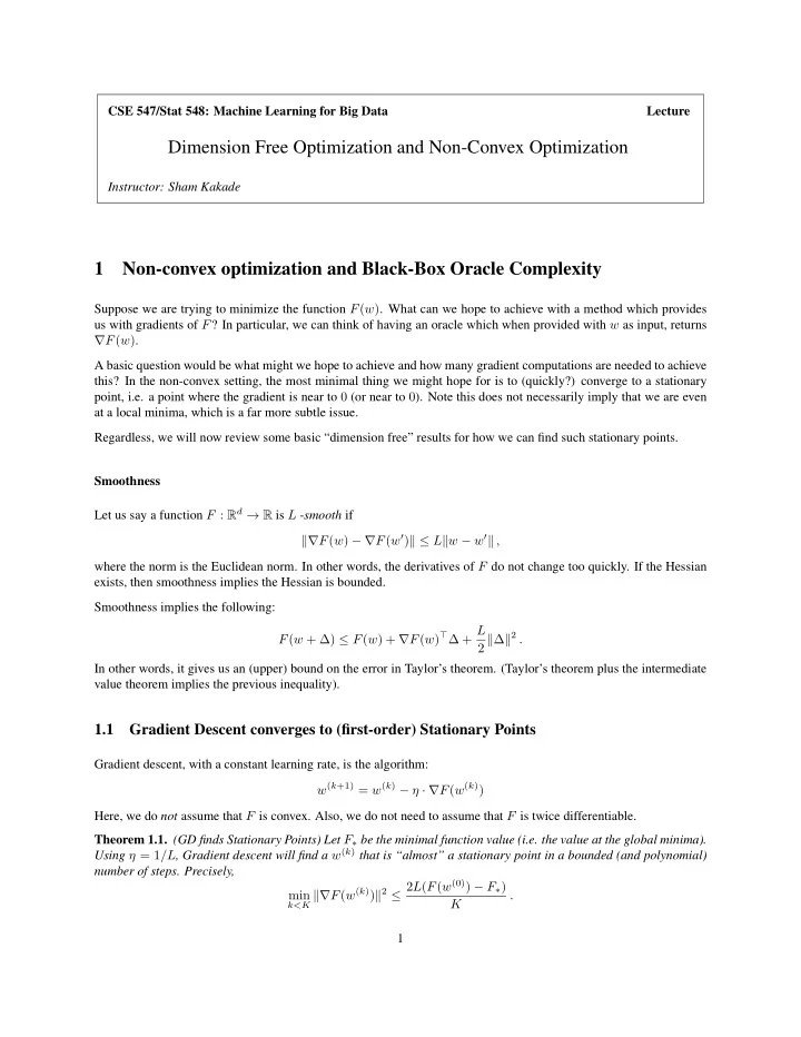
CSE 547/Stat 548: Machine Learning for Big Data Lecture Dimension Free Optimization and Non-Convex Optimization Instructor: Sham Kakade 1 Non-convex optimization and Black-Box Oracle Complexity Suppose we are trying to minimize the function F ( w ) . What can we hope to achieve with a method which provides us with gradients of F ? In particular, we can think of having an oracle which when provided with w as input, returns ∇ F ( w ) . A basic question would be what might we hope to achieve and how many gradient computations are needed to achieve this? In the non-convex setting, the most minimal thing we might hope for is to (quickly?) converge to a stationary point, i.e. a point where the gradient is near to 0 (or near to 0 ). Note this does not necessarily imply that we are even at a local minima, which is a far more subtle issue. Regardless, we will now review some basic “dimension free” results for how we can find such stationary points. Smoothness Let us say a function F : R d → R is L - smooth if �∇ F ( w ) − ∇ F ( w ′ ) � ≤ L � w − w ′ � , where the norm is the Euclidean norm. In other words, the derivatives of F do not change too quickly. If the Hessian exists, then smoothness implies the Hessian is bounded. Smoothness implies the following: F ( w + ∆) ≤ F ( w ) + ∇ F ( w ) ⊤ ∆ + L 2 � ∆ � 2 . In other words, it gives us an (upper) bound on the error in Taylor’s theorem. (Taylor’s theorem plus the intermediate value theorem implies the previous inequality). 1.1 Gradient Descent converges to (first-order) Stationary Points Gradient descent, with a constant learning rate, is the algorithm: w ( k +1) = w ( k ) − η · ∇ F ( w ( k ) ) Here, we do not assume that F is convex. Also, we do not need to assume that F is twice differentiable. Theorem 1.1. (GD finds Stationary Points) Let F ∗ be the minimal function value (i.e. the value at the global minima). Using η = 1 /L , Gradient descent will find a w ( k ) that is “almost” a stationary point in a bounded (and polynomial) number of steps. Precisely, k<K �∇ F ( w ( k ) ) � 2 ≤ 2 L ( F ( w (0) ) − F ∗ ) min . K 1

(Note that �∇ F ( w ( k ) ) � may not be decreasing at every step.) Proof. Smoothness implies that: F ( w ( k +1) ) ≤ F ( w ( k ) ) − η �∇ F ( w ( k ) ) � 2 + 1 2 η 2 L �∇ F ( w ( k ) ) � 2 Our setting of η implies: F ( w ( k +1) ) ≤ F ( w ( k ) ) − 1 2 L �∇ F ( w ( k ) ) � 2 Using that the min is less than the average and by summing over k , K − 1 0 ≤ k<K �∇ F ( w ( k ) ) � 2 ≤ 1 � �∇ F ( w ( k ) ) � 2 min K t =0 K − 1 ≤ 2 L � � � F ( w ( k ) ) − F ( w ( k +1) ) K t =0 = 2 L � � F ( w (0) ) − F ( w ( K ) ) K ≤ 2 L � � F ( w (0) ) − F ∗ ) K which completes the proof. 1.2 Gradient Descent, plus a little noise, converges to (second order) Stationary Points See the readings. 1.3 SGD finds Stationary Points For SGD, we provide the argument due to [Ghadimi and Lan(2013)] Assume we have an N sized training set T . Define: F ( w ) = 1 � ℓ ( w, ( x, y )) N ( x,y ) ∈T Gradient descent, with a constant learning rate, is the algorithm: 1. Initialize at some w (0) . 2. Sample ( x, y ) uniformly at random from the set T 3. Update the parameters: w ( k +1) = w ( k ) − η k · ∇ ℓ ( w ( k ) , ( x, y )) and go back to 2 . Here, we do not assume that F is convex. Also, we do not need to assume that F is twice differentiable. 2

Theorem 1.2. Let us run SGD for K steps. Suppose our gradient is bounded as follows: ∇ ℓ ( w, ( x, y )) ≤ B for all w √ � 2( F ( w (0) ) − F ∗ ) and examples ( x, y ) . Assume our (constant) learning rate is η k = η = c/ K , where c = ). We have LB 2 that: � 2( F ( w (0) ) − F ∗ ) L k<K E [ �∇ F ( w ( k ) ) � 2 ] ≤ B min K where the expectation is with respect to the random sampling in our algorithm. It is interesting to compare the complexity of SGD with GD. Importantly, note the convergence rate of SGD does not depend on N . Remark: The above bound implicitly assumes we know the end iteration K in advance. Alternatively, we could √ adaptive set η k = O (1 / k ) to obtain the same bound (up to constant factors). The proof is simpler when we know K in advance. � Proof. Denote the sampled gradient at iteration k by ∇ F ( w ( k ) ) . From smoothness of F and the gradient descent update rule, we get, E F ( w ( k +1) ) = E F ( w ( k ) + w ( k +1) − w ( k ) ) � F ( w ( k ) ) + ∇ F ( w ( k ) ) ⊤ ( w ( k +1) − w ( k ) ) + L � 2 � w ( k +1) − w ( k ) � 2 ≤ E � ∇ F ( w ( k ) ) + η 2 L � � � F ( w ( k ) ) − η ∇ F ( w ( k ) ) ⊤ ∇ F ( w ( k ) ) � 2 = E 2 � ≤ E [ F ( w ( k ) )] − ηE �∇ F ( w ( k ) ) � 2 + η 2 LB 2 2 Rearranging gives: + η LB 2 E �∇ F ( w ( k ) ) � 2 ≤ 1 � � E [ F ( w ( k ) )] − E [ F ( w ( k +1) )] η 2 Summing over k gives: K − 1 0 ≤ k<K E �∇ F ( w ( k ) ) � 2 ≤ 1 � E �∇ F ( w ( k ) ) � 2 min K t =0 + η LB 2 1 � � E [ F ( w (0) )] − E [ F ( w ( K ) )] ≤ Kη 2 + η LB 2 1 � � F ( w (0) ) − F ∗ ≤ Kη 2 and our choice of η leads to the result. Note that our choice of η is the one which minimizes this upper bound. 1.4 Adaptive Gradient Methods This is an argument due Krishna Pillutla. Let us consider the gradient descent iteration w ( k +1) = w ( k ) − η k ∇ F ( w ( k ) ) . In this section, we shall analyze the �� k effect of setting step-sizes as η k = C/ j =0 �∇ F ( w ( j ) ) � 2 , where C is a constant. 3

Theorem 1.3. Suppose F is L -smooth and bounded from below by F ∗ . Then, gradient descent with adaptive step-sizes �� k j =0 �∇ F ( w ( j ) ) � 2 produces a sequence of iterates { w ( k ) } k ≥ 0 such that η k = C/ C 2 · ( F ( w (0) ) − F ∗ ) 2 j ≤ k �∇ F ( w ( j ) ) � 2 ≤ 4 min k + 1 provided C ≤ �∇ F ( w (0) ) � . L Proof. Define ∆ k := F ( w ( k ) ) − F ∗ . From smoothness of F and the gradient descent update rule, we get, ∆ k +1 ≤ ∆ k + ∇ F ( w ( k ) ) ⊤ ( w ( k +1) − w ( k ) ) + L 2 � w ( k +1) − w ( k ) � 2 � η k − L � = ∆ k − �∇ F ( w ( k ) ) � 2 2 η 2 . k If the gradient is non-zero, the method produces a stricts decrease in the objective value if η k < 2 /L . Moreover, if 2 η 2 k ) ≥ η k η k ≤ 1 /L , we have that ( η k − L 2 . Note that the condition on C ensures this for all k . And so, we get �∇ F ( w ( k ) ) � 2 ≤ 2 (∆ k − ∆ k +1 ) . η k Summing up, and noting that 0 ≤ ∆ k ≤ ∆ 0 , we get � 1   k k �  ∆ 0 1 − ∆ k +1  ≤ 2 �∇ F ( w ( j ) ) � 2 ≤ 2 � � + ∆ j − ∆ 0 . η 0 η j η j − 1 η k η k j =0 j =1 Plugging in the rule to set η k , k �∇ f ( w ( j ) ) � 2 ≤ 4 � C 2 ∆ 2 0 . j =0 Now divide by k + 1 and note that the minimum is no larger than the average to complete the proof. References [Ghadimi and Lan(2013)] Saeed Ghadimi and Guanghui Lan. Stochastic first- and zeroth-order methods for noncon- vex stochastic programming. SIAM Journal on Optimization , 23(4):2341–2368, 2013. 4