Determinism vs randomness There are two main kinds of processes in - PowerPoint PPT Presentation

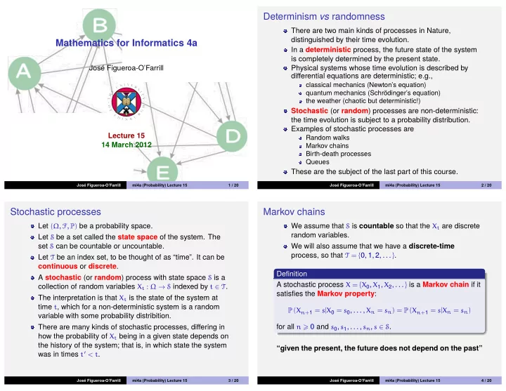
Determinism vs randomness There are two main kinds of processes in Nature, distinguished by their time evolution. Mathematics for Informatics 4a In a deterministic process, the future state of the system is completely determined by the present state. José Figueroa-O’Farrill Physical systems whose time evolution is described by differential equations are deterministic; e.g., classical mechanics (Newton’s equation) quantum mechanics (Schrödinger’s equation) the weather (chaotic but deterministic!) Stochastic (or random ) processes are non-deterministic: the time evolution is subject to a probability distribution. Examples of stochastic processes are Lecture 15 Random walks 14 March 2012 Markov chains Birth-death processes Queues These are the subject of the last part of this course. José Figueroa-O’Farrill mi4a (Probability) Lecture 15 1 / 20 José Figueroa-O’Farrill mi4a (Probability) Lecture 15 2 / 20 Stochastic processes Markov chains Let ( Ω , F , P ) be a probability space. We assume that S is countable so that the X t are discrete random variables. Let S be a set called the state space of the system. The set S can be countable or uncountable. We will also assume that we have a discrete-time process, so that T = { 0, 1, 2, . . . } . Let T be an index set, to be thought of as “time”. It can be continuous or discrete . Definition A stochastic (or random ) process with state space S is a A stochastic process X = { X 0 , X 1 , X 2 , . . . } is a Markov chain if it collection of random variables X t : Ω → S indexed by t ∈ T . satisfies the Markov property : The interpretation is that X t is the state of the system at time t , which for a non-deterministic system is a random P ( X n + 1 = s | X 0 = s 0 , . . . , X n = s n ) = P ( X n + 1 = s | X n = s n ) variable with some probability distribition. for all n � 0 and s 0 , s 1 , . . . , s n , s ∈ S . There are many kinds of stochastic processes, differing in how the probability of X t being in a given state depends on the history of the system; that is, in which state the system “given the present, the future does not depend on the past” was in times t ′ < t . José Figueroa-O’Farrill mi4a (Probability) Lecture 15 3 / 20 José Figueroa-O’Farrill mi4a (Probability) Lecture 15 4 / 20

Random walks Proposition Consider a particle moving on the integer lattice in R : The sequence { X 0 , X 1 , X 2 , . . . } exhibits spatial homogeneity : q p P ( X n = j | X 0 = a ) = P ( X n = j + b | X 0 = a + b ) i − 1 i i + 1 Proof. Therefore S = Z and J i are independent random variables with � n � � P ( J i = 1 ) = p P ( J i = − 1 ) = q = 1 − p P ( X n = j | X 0 = a ) = P J i = j − a i = 1 and also Let X n denote the position of the particle at time n , so that � n � � n P ( X n = j + b | X 0 = a + b ) = P J i = j + b − ( a + b ) = j − a � X n = X 0 + J i i = 1 i = 1 José Figueroa-O’Farrill mi4a (Probability) Lecture 15 5 / 20 José Figueroa-O’Farrill mi4a (Probability) Lecture 15 6 / 20 Proposition Proposition The sequence { X 0 , X 1 , X 2 , . . . } exhibits temporal homogeneity : The sequence { X 0 , X 1 , X 2 , . . . } exhibits the Markov property : P ( X m + n = j | X 0 = i 0 , . . . , X m = i m ) = P ( X m + n = j | X m = i m ) P ( X n = j | X 0 = a ) = P ( X n + m = j | X m = a ) Proof. Proof. � n This follows because � � P ( X n = j | X 0 = a ) = P J i = j − a n � i = 1 X m + n = X m + J i whereas i = m + 1   m + n so X m + n does not depend explicitly on the X j for j < m . � P ( X n + m = j | X m = a ) = P J i = j − a   i = m + 1 but the J i are i.i.d. José Figueroa-O’Farrill mi4a (Probability) Lecture 15 7 / 20 José Figueroa-O’Farrill mi4a (Probability) Lecture 15 8 / 20

Example (Gambler’s ruin) Example (Gambler’s ruin – continued) A gambler starts with £ k and plays a game in which a fair coin Letting p k = P k ( R ) , we have the following difference equation: is tossed repeatedly: winning £1 if heads and − £1 if tails. The p k = 1 p 0 = 1 p N = 0 2 ( p k + 1 + p k − 1 ) game stops when the gambler’s fortune is either £ N ( N > k ) or £0. What is the probability that the gambler is ultimately ruined? Let a k = p k − p k − 1 . Then This is an example of a random walk on a finite set { 0, 1, 2, . . . , N } . Let R denote the event that the gambler is a k − a k − 1 = p k − p k − 1 − ( p k − 1 − p k − 2 ) eventually ruined and let H and T denote the events that the = p k − 2 p k − 1 + p k − 2 first toss is heads and tails, respectively. Let P k ( R ) denote the = p k − ( p k + p k − 2 ) + p k − 2 = 0 probability that gambler is eventually ruined starting with £ k . Then Therefore a k = a 1 for all k and hence P k ( R ) = P k ( R | H ) P ( H ) + P k ( R | T ) P ( T ) but clearly P k ( R | H ) = P k + 1 ( R ) and P k ( R | T ) = P k − 1 ( R ) , whence p k = a 1 + p k − 1 = 2 a 1 + p k − 2 = · · · = ka 1 + p 0 P k ( R ) = 1 2 P k + 1 ( R ) + 1 Since p 0 = 1 and p N = 0, we find a 1 = − 1 N , whence p k = 1 − k N . 2 P k − 1 ( R ) José Figueroa-O’Farrill mi4a (Probability) Lecture 15 9 / 20 José Figueroa-O’Farrill mi4a (Probability) Lecture 15 10 / 20 Example (Gambler’s ruin – continued) Example (Gambler’s ruin – continued) What about if the coin is not fair? Imposing the boundary conditions Let P ( H ) = p and P ( T ) = q = 1 − p , with p � = q . Now � N � q 1 = p 0 = c 1 + c 2 0 = p N = c 1 + c 2 p p k = pp k + 1 + qp k − 1 1 � k � N − 1 whence with the same boundary conditions p 0 = 1 and p N = 0. Try a 1 � N � q c 1 = − c 2 c 2 = solution p k = θ k for some θ . Then p � N � q 1 − p θ k = pθ k + 1 + qθ k − 1 = ⇒ pθ 2 − θ + q = 0 and hence with roots θ 1 = 1 and θ 2 = q p . The general solution is then � N � k � k � N � � � � q q q q − p p p p p k = − � N + � N = p k = c 1 θ k 1 + c 2 θ k � N � � � q q q 2 1 − 1 − 1 − p p p for some c 1 , c 2 which are determined by p 0 = 1 and p N = 0. José Figueroa-O’Farrill mi4a (Probability) Lecture 15 11 / 20 José Figueroa-O’Farrill mi4a (Probability) Lecture 15 12 / 20

Transition matrix Theorem Let’s go back to the case of a general Markov chain The transition matrix of a Markov chain is stochastic ; that is, { X 0 , X 1 , X 2 , . . . } . p ij � 0 1 Since S is countable we will assume it is a subset of Z . � j p ij = 1 for all i (i.e., rows sum to 1 ) 2 The evolution of a Markov chain is described by its transition probabilities Proof. P ( X n + 1 = j | X n = i ) This is obvious since the p ij are probabilities. 1 We will make the additional assumption of temporal 2 � � homogeneity: p ij = P ( X n + 1 = j | X n = i ) = 1 j j P ( X n + 1 = j | X n = i ) = P ( X 1 = j | X 0 = i ) since X n + 1 must take some value. Therefore the transition probabilities are encoded in a transition matrix P = ( p ij ) , where p ij = P ( X n + 1 = j | X n = i ) José Figueroa-O’Farrill mi4a (Probability) Lecture 15 13 / 20 José Figueroa-O’Farrill mi4a (Probability) Lecture 15 14 / 20 Example Example (Continued) Let X n denote the state of a computer at the start of the n th We often represent Markov chains graphically; e.g., day. The computer can be in either of two states: X n = 0 if it is q broken or X n = 1 if in working order. Let π n ( 0 ) = P ( X n = 0 ) and π n ( 1 ) = P ( X n = 1 ) = 1 − π n ( 0 ) . 1 − p 0 1 1 − q Let the transition probabilities be p P ( X n + 1 = 1 | X n = 0 ) = p P ( X n + 1 = 0 | X n = 0 ) = 1 − p which allows us to read the transition probabilities at a glance P ( X n + 1 = 0 | X n = 1 ) = q P ( X n + 1 = 1 | X n = 1 ) = 1 − q and write down the transition matrix: (Notice that p + q need not equal 1!) � 0 → 0 � � 1 − p � 0 → 1 p Therefore the transition matrix is P = = 1 → 0 1 → 1 1 − q q � 1 − p � p P = 1 − q q A typical question is: What is P ( X n + 1 = 0 ) ? We will answer this naively at first. José Figueroa-O’Farrill mi4a (Probability) Lecture 15 15 / 20 José Figueroa-O’Farrill mi4a (Probability) Lecture 15 16 / 20