Determinants of Social Discount Rate, general case The resulting - PowerPoint PPT Presentation
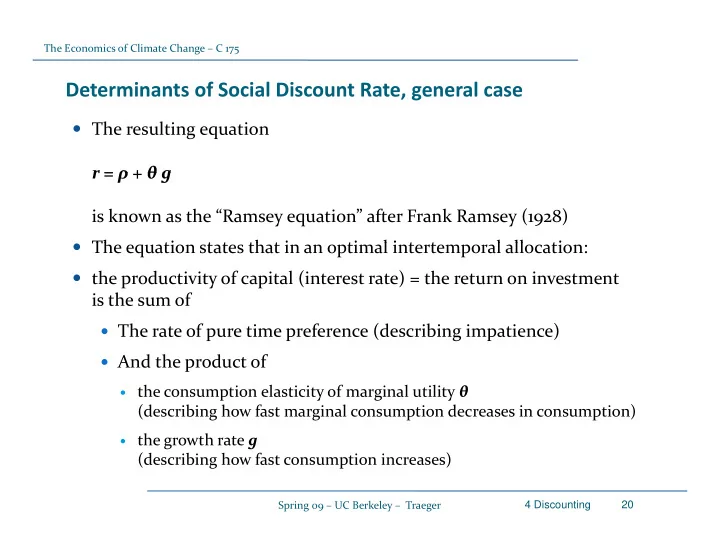
The Economics of Climate Change C 175 Determinants of Social Discount Rate, general case The resulting equation r = + g r = + g is known as the Ramsey equation after Frank Ramsey (1928) The equation states that in an
The Economics of Climate Change – C 175 Determinants of Social Discount Rate, general case The resulting equation r = ρ + θ g r = ρ + θ g is known as the “Ramsey equation” after Frank Ramsey (1928) The equation states that in an optimal intertemporal allocation: Th ti t t th t i ti l i t t l ll ti the productivity of capital (interest rate) = the return on investment is the sum of The rate of pure time preference (describing impatience) And the product of the consumption elasticity of marginal utility θ (describing how fast marginal consumption decreases in consumption) the growth rate g (d (describing how fast consumption increases) b h f ) Spring 09 – UC Berkeley – Traeger 4 Discounting 20
The Economics of Climate Change – C 175 The Economics of Climate Change C 175 ‐ Christian Traeger 75 g Part 4: Discounting continued Lecture 17 Background still Cameron Hepburn’s (2006), “Discounting climate change damages: Working note for the Stern review”. 3 Instruments 21 Spring 09 – UC Berkeley – Traeger
The Economics of Climate Change – C 175 Review Problem: How to compare costs and benefits that occur at different points in time? time? Economic solution concept involves: Discounting: Describes the valuation in present day terms of future g outcomes (damages, costs, benefits, utility values) Cost Benefit analysis: Assess costs and benefits in monetary units Assess costs and benefits in monetary units Express all benefits and costs in present value terms Net present value NPV : Support a project if present value benefits exceed present value costs S t j t if t l b fit d t l t B C T t t NPV r ) t t 0 ( ( 1 1 r ) 4 Discounting 22 Spring 09 – UC Berkeley – Traeger
The Economics of Climate Change – C 175 Answer to Homework Example II Cost Benefit analysis: Consider the two modified projects and a discount rate of 5%. Benefits (in $) Year 0 1 2 3 Project A Project A -30 30 20 20 10 10 10 10 Project B -30 10 20 20 Assume you only have $30 that you can invest in the first period. Which project would you invest in? NPV A = ‐ $30+$20/(1,05) +$10/(1,05) 2 +$10/(1,05) 3 = $6.76 $30+$20/(1 05) +$10/(1 05) 2 +$10/(1 05) 3 $6 76 NPV NPV B = ‐ $30+$10/(1,05) +$20/(1,05) 2 +$20/(1,05) 3 = $14.94 Project B because NPV B >NPV A j B A Spring 09 – UC Berkeley – Traeger 4 Discounting 23
The Economics of Climate Change – C 175 Review: How to find the discount rate? Recall importance of discounting for long time horizons: At a 10% discount rate $ 1 Mio in 150 years have present value of 1% discount rate $ 1 Mio in 150 years have present value of $ 225 000 % di Mi i h l f High discount rate implies A dollar today is much more valuable than a dollar tomorrow Hard to justify climate policy where costs occur today but benefits (abated damages) accrue later How do we find the “correct” discount rate? Market Intertest Ra te ‐ > BUT: might not exist for long time horizons or not represent “correct” information (market failures, responsibilities for future generations) Identify components of the Social Discount Rate d if f h S i l Di R Spring 09 – UC Berkeley – Traeger 4 Discounting 24
The Economics of Climate Change – C 175 Review: The Social Discount Rate We have derived how the optimal real interest rate should be composed if markets were perfect and represented all information: Then: MRS MRT Then: MRS = MRT (Marginal rate of substitution = Marginal rate of transformation) Where: Good 1 = consumption today G d i d Good 2 = consumption tomorrow Result is the Ramsey equation: r = ρ + θ g y q ρ g We derived the equation for a two period setting, but holds in general, also in continuous time: r(t) = ρ + θ ( x(t) ) g(t) Remark: θ (x(t)) is determined by the utility function. If utility is a power function (i e x α ) then θ α independent of x(t) (i.e. x α ) then θ = α independent of x(t) . Spring 09 – UC Berkeley – Traeger 4 Discounting 25
The Economics of Climate Change – C 175 Review: Determinants of Social Discount Rate Ramsey equation: r(t) = ρ + θ g(t) Optimal productivity of capital ( r ) equals p p y p ( ) q The rate of pure time preference ( ρ ) (describing impatience) And the product of the consumption elasticity of marginal utility θ (describing how fast marginal utility decreases in consumption) Relative change of marginal utility Relative change of marginal utility dU ' ( X ) under a relative change of consumption. U ' ' ( X ) X U ' ( X ) or dX U ' ( X ) By how many percent does marginal X X utility change if consumption increases by one percent the growth rate g (describing how fast consumption increases) ( g p ) Spring 09 – UC Berkeley – Traeger 4 Discounting 26
The Economics of Climate Change – C 175 So what’s the rate? ‐ Normative vs Descriptive Two approaches Descriptive : Observe r(t) and g(t) . Either in market or in experiments. Different combinations of ρ and θ are generally compatible with these observations. D t Determining θ by observation is harder but would identify corresponding ρ . i i θ b b ti i h d b t ld id tif di Prescriptive : Start with deciding on ρ and θ . Then growth rate g(t) determines the corresponding real interest rate r(t) . Arguments for picking ρ and θ di l i ( ) A f i ki d θ generally rely on ethical reasoning. Spring 09 – UC Berkeley – Traeger 4 Discounting 27
The Economics of Climate Change – C 175 So what’s the rate? ‐ Pure Time Preference ρ : Some opinions that it should be zero: Ramsey (1928) describes placing different weights upon the utility of diff different generations, as ‘ ethically indefensible ’. i ‘ hi ll i d f ibl ’ Harrod (1948) stated that discounting utility represented a ‘ polite expression for rapacity and the conquest of reason by passion ’. … Stern Review (2007) – to be encountered in integrated assessment part ‐ > These are mostly ethical arguments and thus prescriptive Th l hi l d h i i Remark: Ramsey equation including (undetermined!) parameter ρ can be derived from y q g p ρ axioms, i.e. assumptions on behavior rather than starting with our utility model Changing the axioms to include risk attitude in a more comprehensive way can eliminate ρ , that is, make it zero starting from assumptions on rational and consistent behavior rather than for ethical reasons (paper on my homepage) i b h i h h f hi l ( h ) Spring 09 – UC Berkeley – Traeger 4 Discounting 28
The Economics of Climate Change – C 175 So what’s the rate? ‐ Descriptive Descriptive take on ρ : By reverse engineering from observations economists often take values between 2% and 3% . Similarly θ is engineered to be between 1 and 4. Si il l i i d b b d Remark: The high (& even higher) values of θ are obtained from risk studies where θ also represents risk aversion rather than just reduction in marginal utility from growth over time. The growth rate g is observed and predicted to be approximately in the range 1% to 3% The real interest rate employed as observed rate ranges approximately from The real interest rate employed as observed rate ranges approximately from 2% to 7% A convenient example of somewhat reasonable values (Weitzman 2007) ρ =2%, θ =2, g=2%, r=6% Other examples ‐ Stern review (2007) Nordhaus (2007) – on problem set Other examples Stern review (2007), Nordhaus (2007) on problem set. Spring 09 – UC Berkeley – Traeger 4 Discounting 29
The Economics of Climate Change – C 175 So what’s the rate? ‐ Prescriptive ρ : possibly zero for ethical reasons as proposed on earlier slide θ : Normative/ethical information conveyed: Equalizing consumption across generations If θ =0 , then more or less consumption in the future does not change willingness to invest ( r independent of growth rate g ) change willingness to invest ( r independent of growth rate g ) If θ is large, then with positive growth ‐ > not willing to invest in future (future generations have more anyhow) If θ is large, then with negative growth ‐ > very willing to invest in future (future generations are poorer than today’s) Proposed range for θ ranges from 1 to 4 Proposed range for θ ranges from 1 to 4 Remark: Willing to invest in future = low real interest rate in optimal allocation. Spring 09 – UC Berkeley – Traeger 4 Discounting 30
The Economics of Climate Change – C 175 Distributive Justice Excursion: Rawls theory of justice applied to intertemporal distribution Would set ρ to zero and increase θ to ∞ More generally, an egalitarian perspective with respect to time yields ρ small and thus r small distribution across generations (stripping off the time dimension) distribution across generations (stripping off the time dimension) yields θ large and thus r large if positive growth Spring 09 – UC Berkeley – Traeger 4 Discounting 31
Recommend
More recommend
Explore More Topics
Stay informed with curated content and fresh updates.
