Derivative Free Optimization Optimization and AMS Masters - - PDF document

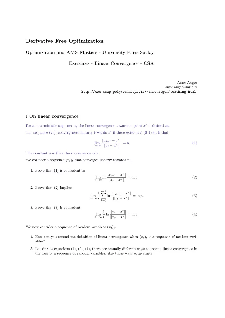
Derivative Free Optimization Optimization and AMS Masters - University Paris Saclay Exercices - Linear Convergence - CSA Anne Auger anne.auger@inria.fr http://www.cmap.polytechnique.fr/~anne.auger/teaching.html I On linear convergence For a deterministic sequence x t the linear convergence towards a point x ∗ is defined as: The sequence ( x t ) t convergences linearly towards x ∗ if there exists µ ∈ (0 , 1) such that � x t +1 − x ∗ � lim = µ (1) � x t − x ∗ � t →∞ The constant µ is then the convergence rate. We consider a sequence ( x t ) t that converges linearly towards x ∗ . 1. Prove that (1) is equivalent to t →∞ ln � x t +1 − x ∗ � lim = ln µ (2) � x t − x ∗ � 2. Prove that (2) implies t − 1 ln � x k +1 − x ∗ � 1 � lim = ln µ (3) t � x k − x ∗ � t →∞ k =0 3. Prove that (3) is equivalent t ln � x t − x ∗ � 1 lim � x 0 − x ∗ � = ln µ (4) t →∞ We now consider a sequence of random variables ( x t ) t . 4. How can you extend the definition of linear convergence when ( x t ) t is a sequence of random vari- ables? 5. Looking at equations (1), (2), (4), there are actually different ways to extend linear convergence in the case of a sequence of random variables. Are those ways equivalent?

[This is the answer to questions 4. and 5. please do not read before to have thought about an answer to 4. and 5.] For a sequence of random variables ( x t ) t . We can define linear convergence by considering the expected log progress, that is the sequence converges linearly if � � ln � x t +1 − x ∗ � t →∞ E lim = ln µ , � x t − x ∗ � Remark that in general � � � � x t +1 − x ∗ � � ln � x t +1 − x ∗ � E � = ln E � x t − x ∗ � � x t − x ∗ � � � � x t +1 − x ∗ � and thus defining linear convergence via lim t E would not be equivalent contrary to the � x t − x ∗ � deterministic case. If we want to define the almost sure linear convergence we cannot use directly (1) or (2) as � x t +1 − x ∗ � or � x t − x ∗ � ln � x t +1 − x ∗ � are random variables that will not convergence almost surely to a constant. We therefore � x t − x ∗ � have to resort to (5) and define the almost sure linear convergence of a sequence of random variables as t ln � x t − x ∗ � 1 lim � x 0 − x ∗ � = ln µ a.s. (5) t →∞ 6. When you investigate the convergence of an algorithm numerically, how can you visualize whether (5) holds? What should you plot? [hint: think about the plots you have done when looking at the convergence of the (1+1)-ES with one-fifth success rule] II Cumulative Step-size Adaptation (CSA) In this exercice, we want to understand the normalization constants in the CSA algorithm and how they implement the idea explained during the class. The pseudo-code of the ( µ/µ, λ )-ES with CSA step-size adaption is given in the following. [Objective: minimize f : R n → R ] 1. Initialize σ 0 > 0, m 0 ∈ R n , p 0 = 0, t = 0 2. set w 1 ≥ w 2 ≥ . . . w µ ≥ 0 with � w i = 1; µ eff = 1 / � w 2 i , 0 < c σ < 1 (typically c σ ≈ 4 /n ), d σ > 0 3. while not terminate 4. Sample λ independent candidate solutions : X i t +1 = m t + σ t y i 5. t +1 for i = 1 . . . λ with ( y i t +1 ) 1 ≤ i ≤ λ i.i.d. following N ( 0 , I d ) 6. Evaluate and rank solutions: 7. f ( X 1: λ t +1 ) ≤ . . . ≤ f ( X λ : λ 8. t +1 ) Update the mean vector: 9. µ � w i y i : λ m t +1 = m t + σ t 10. t +1 i =1 � �� � y w t +1 11. Update the path: 1 − (1 − c σ ) 2 √ µ eff y w � p t +1 = (1 − c σ ) p t + 12. t +1 Update the step-size: 13. � � �� � p σ � c σ σ t +1 = σ t exp E [ �N (0 ,I d ) � ] − 1 14. d σ t=t+1 15. 1. Assume that the objective function f is random, i.e. for instance f ( X i t +1 ) i are i.i.d. according to U [0 , 1] . What is the distribution of √ µ eff y w t +1 ? 2

2. Assume that p t ∼ N (0 , I d ) and that the selection is random, show that p t +1 ∼ N (0 , I d ) 3. Deduce that under random selection E [ln σ t +1 | σ t ] = ln σ t and then that the expected log step-size is constant. 3