Derandomised lattice rules for high dimensional integration Ian - PowerPoint PPT Presentation
Derandomised lattice rules for high dimensional integration Ian Sloan i.sloan@unsw.edu.au University of New South Wales, Sydney, Australia RICAM, December, 2018 Joint with Yoshihito Kazashi (EPFL) and Frances Kuo (UNSW) We want to approximate
Derandomised lattice rules for high dimensional integration Ian Sloan i.sloan@unsw.edu.au University of New South Wales, Sydney, Australia RICAM, December, 2018 Joint with Yoshihito Kazashi (EPFL) and Frances Kuo (UNSW)
We want to approximate � 1 � 1 I s ( f ) := . . . f ( x 1 , . . . , x s )d x 1 . . . d x s 0 0 � = [0 , 1] s f (x)dx . In practice this usually means that some transformation to the unit cube has already been carried out. And s may be large.
Quasi-Monte Carlo (QMC) For QMC we take N I s ( f ) ≈ Q N,s ( f ) := 1 � f (t k ) , N k =1 with t 1 , . . . , t N deterministic (and cleverly chosen). How to choose t 1 , . . . , t N ? Low discrepancy points (Halton, Sobol ′ , Faure, Niederreiter, . . . ) Lattice rules (Korobov, Hlawka, Zaremba, Hua).
We consider only the simplest kind of lattice rule, given by N Q N,s (z; f ) = 1 k z �� �� � f , N N k =1 where z ∈ { 1 , . . . , N − 1 } s = Z s N , and the braces mean that each component of the s -vector in the braces is to be replaced by its fractional part. The corresponding shifted lattice rule is N Q N,s (z , ∆; f ) = 1 �� k z �� � f N + ∆ , N k =1 where ∆ ∈ [0 , 1) s .
Example of lattice & shifted lattice rules N = 34 , z = (1 , 21) N = 34 , z = (1 , 21) , ∆ = (0 . 8 , 0 . 1) 1 1 • • • • • • • • • • • • • • • • • • • • • • • • • • • • • • • • • • • • • • • • • • • • • • • • • • • • • • • • • • • • • • • • • • 0 0 • • 0 1 0 1
How to choose z and ∆ ? Recall the shifted lattice rule: N N,s, z , ∆ ( f ) = 1 �� k z �� � Q lattice ∆ ∈ [0 , 1) s , f N + ∆ , N k =1 Here are three possible strategies: Choose ∆ randomly , from a uniform distribution on [0 , 1] s . Then find the best possible choice of z , by finding good values of z 1 , z 2 , . . . , z s one after the other (“CBC”), by minimising some worst-case error . Make an inspired choice of ∆ , eg ∆ = 0 . Then choose z 1 , z 2 , . . . , z s by CBC. Choose z 1 , ∆ 1 , z 2 , ∆ 2 . . . , z s , ∆ s by a more general CBC.
Choosing ∆ randomly There are big advantages in choosing ∆ randomly : Like Monte Carlo, this family is an unbiased estimator of I s ( f ) . For free we get an estimate of the error – in practice we choose say 25 random shifts, and evaluate the lattice rule with a given generating vector z for each shift. Then the mean gives an estimate of the integral, and the spread gives us an estimate of the error. A good z can be constructed by minimising the shift-averaged worst-case error over z 1 , z 2 , , . . . , z s successively – “CBC”. There is excellent theoretical justification (Kuo) and fast implementation (Nuyens). (More about randomly shifted lattice rules later.)
Worst-case error The worst-case error of a given QMC rule with points t 1 , t 2 , . . . t N , in some Hilbert space H s , is e s ( N ; t 1 , . . . , t N ) N � [0 , 1) s f (x) dx − 1 � � � � � := sup f (t k } ) � , � � N � f ∈ H s , � f � Hs ≤ 1 k =1
Choosing the function space H s We take the space H s to be a reproducing kernel Hilbert space . with a kernel K : K ( · , x) ∈ H s ∀ x ∈ [0 , 1) s , K (x , y) = K (y , x) , ( f, K ( · , x)) H s = f (x) ∀ f ∈ H s , ∀ x . For every RKHS it is well known that � � e 2 s ( N ; t 1 , . . . , t N ) = [0 , 1] s K (x , y) dx dy [0 , 1] s N N N − 2 1 � � � � [0 , 1] s K (t k , x) dx + K (t k , t k ′ ) , N 2 N k ′ =1 k =1 k =1
Specialising: In particular we choose the RKHS to be H s,γ with kernel � � K s,γ (x , y) = γ u η ( x j , y j ) , j ∈ u u ⊆{ 1: s } where � �� � η ( x, y ) := 1 x − 1 y − 1 2 B 2 ( | x − y | ) + , x, y ∈ [0 , 1] . 2 2 Here B 2 ( x ) = x 2 − x + 1 / 6 . This implies � for any y ∈ [0 , 1] s , [0 , 1] s K (x , y) dx = 1 and hence the simpler formula N N 1 e 2 � � s ( N ; t 1 , . . . , t N ) = K (t k , t k ′ ) − 1 . N 2 k ′ =1 k =1
What is this space? It is well known that this is a weighted “unanchored” Hilbert space, a space of functions with square integrable mixed first derivatives on [0 , 1] s , with squared norm � f � 2 H s,γ := � 2 �� ∂ | u | f � � γ − 1 (x u ; x { 1: s }\ u ) dx { 1: s }\ u dy u , u ∂ x u [0 , 1] | u | [0 , 1] s −| u | u ⊆{ 1: s } The γ u are “weights”, with γ ∅ = 1 . Example: γ u = � j ∈ u γ j , for some γ 1 ≥ γ 2 ≥ . . . > 0 . Weights are essential for “tractability” (IHS and H Wo´ zniakowski ’98)
For this space, since K s (x , y) = � � u γ u j ∈ u η ( x j , y j ) , we have � e 2 γ u e 2 s ( N ; z , ∆) = u ( N ; z u , ∆) , ∅� = u ⊆{ 1: s } where for u ⊆ { 1 : s } and z u := ( z j ) j ∈ u , N N � k ′ z j �� �� 1 � 1 � kz j � � � � � e 2 � � u ( N ; z u , ∆) := 2 B 2 − � � N 2 N N � � k ′ =1 k =1 j ∈ u � �� k ′ z j �� kz j − 1 − 1 � � � � + N + ∆ + ∆ . 2 N 2 This worst-case error is easily computable for reasonable weights (such as product weights γ u = � j ∈ u γ j ).
For the case of random shifts For the case of random shifts the relevant quantity is the shift-averaged worst-case error , � e sh 2 [0 , 1] s e 2 ( N ; z) = s ( N ; z , ∆)d∆ s N N � k ′ z j 1 �� � kz j �� � � � � � � � � = γ u B 2 − � � N 2 N N � � k ′ =1 k =1 j ∈ u ∅� = u ⊆{ 1: s } We used this fact, important to us later: � 1 { x + ∆ } − 1 { y + ∆ } − 1 d∆ = 1 � � � � 2 B 2 ( | x − y | ) , 2 2 0 � 1 η ( x, y )d∆ = 1 2 B 2 ( | x − y | ) + 1 = ⇒ 2 B 2 ( | x − y | ) 0 = B 2 ( | x − y | ) x, y ∈ [0 , 1] .
For the case of random shifts the relevant quantity is the shift-averaged worst-case error , � e sh 2 [0 , 1] s e 2 ( N, z) = s ( N, z , ∆)d∆ s N N � k ′ z j 1 �� � kz j �� � � � � � � � � = γ u B 2 − � � N 2 N N � � k ′ =1 k =1 j ∈ u ∅� = u ⊆{ 1: s } Finding successive z 1 , z 2 , . . . , z s from the set { 1 , . . . , N − 1 } that minimise this expression can be done very efficiently by fast CBC (Nuyens and Cools ...).
Derandomising But there are benefits too in finding a good deterministic shift – sometimes called derandomising . The practical benefit is that we do not always have to make say 25 random shifts, because that is a big extra cost. Of course we do get some “Monte Carlo” benefit by taking 25 random shifts, but the √ expected reduction of the error is of order only 1 / 25 = 1 / 5 , rather than something closer to 1 / 25 .
Using CBC to fix all ∆ j and z j In 2002 S/Kuo/Joe proposed an algorithm to determine successively z 1 , ∆ 1 , z 2 , ∆ 2 , . . . z s , ∆ s . The idea: suppose z 1 , ∆ 1 , . . . , z s − 1 , ∆ s − 1 are already determined. We next choose z s to minimise � 1 e 2 s ( z 1 , ∆ 1 , . . . , z s − 1 , ∆ s − 1 , z s , ∆ s )d∆ s , 0 which can be evaluated explicitly. Then (in principle) choose ∆ s ∈ [0 , 1] to minimise e s ( z 1 , ∆ 1 , . . . , z s − 1 , ∆ s − 1 , z s , ∆ s ) .
That’s not feasible, but ... We can’t search over all values of ∆ s ∈ [0 , 1] , but SKJ 2002 1 2 N , . . . , 2 N − 1 3 showed that we need search over only 2 N , 2 N . Here’s the argument: Suppose that z 1 , ∆ 1 , . . . , z s − 1 , ∆ s − 1 are fixed. It can easily be shown that e 2 s ( z 1 , ∆ 1 , . . . , z s − 1 , ∆ s − 1 , z s , ∆ s ) = e 2 s − 1 ( z 1 , ∆ 1 , . . . , z s − 1 , ∆ s − 1 ) + θ s ( z 1 , ∆ 1 , . . . , z s − 1 , ∆ s − 1 , z s , ∆ s ) ,
e 2 s ( z 1 , ∆ 1 , . . . , z s − 1 , ∆ s − 1 , z s , ∆ s ) = e 2 s − 1 ( z 1 , ∆ 1 , . . . , z s − 1 , ∆ s − 1 ) + θ s ( z 1 , ∆ 1 , . . . , z s − 1 , ∆ s − 1 , z s , ∆ s ) , where for product weights we have s − 1 N N θ s ( z 1 , . . . , ∆ s − 1 , z s , ∆ s ) := γ s � � � (1 + γ j η ( t k,j , t k ′ ,j )) N 2 k ′ =1 k =1 j =1 �� ( k − k ′ ) z s � �� k ′ z s �� kz s � �� � � �� 1 − 1 − 1 × 2 B 2 + N + ∆ s + ∆ s 2 2 N N
The minimiser ∆ ∗ s satisfies s ) ≤ 1 � θ s ( z s , ∆ ∗ θ s ( z s , ∆ s ) N 2 N ,..., 2 N − 1 ∆ s ∈{ 1 2 N , 3 } 2 N � 1 ≤ θ s ( z s , ∆ s )d∆ s . 0 The first inequality holds because ... The 2nd inequality holds because the midpoint rule underestimates � 1 � �� k ′ z s �� kz s � � � − 1 − 1 N + ∆ s + ∆ s d∆ s . 2 2 N 0 The integrand is a piecewise quadratic in ∆ s , with breakpoints at multiples of 1 /N , and positive curvature in between.
And the minimiser z ∗ s satisfies if N is prime � 1 N − 1 1 � θ ( z ∗ s , ∆ ∗ s ) ≤ θ s ( z s , ∆ s )d∆ s N − 1 0 z s =1 N − 1 N N s − 1 �� ( k − k ′ ) z s 1 �� ≤ γ s � � � � (1 + γ j η ( t k,j , t k ′ ,j )) B 2 N 2 N − 1 N z s =1 j =1 k =1 k ′ =1 But B 2 (0) = 1 N − 1 if k = k ′ B 2 ( { ( k − k ′ ) z s 1 6 � } ) = N − 1 N − 1 if k � = k ′ z s =1 6 N s − 1 s ) ≤ γ s (1 + γ j � ⇒ θ ( z ∗ s , ∆ ∗ = 3 ) . 6 N j =1
Recommend
More recommend
Explore More Topics
Stay informed with curated content and fresh updates.
