[PPT] - Deleting an edge 5. Deletioncontraction and graph polynomials For a PowerPoint Presentation

SLIDE 1

✬ ✫ ✩ ✪

Throughout this lecture we assume that G is an undirected graph, possibly with loops and parallel edges. Many basic invariants associated with G can be expressed using a recurrence formula involving deletions and contractions of the edges of G. In this lecture we explore some of these invariants, and express them using a “universal” such invariant, the Tutte polynomial TG(x, y).

✬ ✫ ✩ ✪

Sources for this lecture

The material for this lecture has been prepared with the help of [Big, Chaps. 9–14], [Bol, Chap. X], and [God, Chap. 15]. [Big]

bridge University Press, Cambridge, 1993. [Bol]

as, Modern Graph Theory, Springer, New York NY, 1998. [God]

Algebraic Graph Theory, Springer, New York NY, 2004.

✬ ✫ ✩ ✪

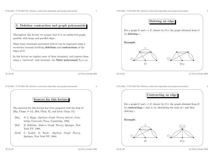
Deleting an edge

For a graph G and e ∈ E, denote by G\e the graph obtained from G by deleting e. Example.

e G G\e

✬ ✫ ✩ ✪

Contracting an edge

For a graph G and e ∈ E, denote by G/e the graph obtained from G by contracting e; that is, by identifying the ends of e and then deleting e. Example.

e G G/e

SLIDE 2

✬ ✫ ✩ ✪

Deletion–contraction trees

Given a graph G, construct a deletion–contraction tree of G recursively as follows. The root of the tree is the graph G. If G has no edges, stop. If all edges of G are loops, and there is a loop e, recursively add the tree of G\e as a child of G. Otherwise, if G all edges of G are either loops or cut-edges, and there is a cut edge e, recursively add the tree of G/e as a child of G. Otherwise, let e be an edge that is neither a loop nor a cut-edge, recursively add the trees of G\e and G/e as children of G.

✬ ✫ ✩ ✪

Example

✬ ✫ ✩ ✪

Deletion–contraction recurrences

Let f be a graph invariant. A deletion–contraction recurrence for f expresses f(G) for a nonempty G in terms of the deletion f(G\e) and the contraction f(G/e) of an edge e ∈ E. Loops and cut-edges are typically treated as special cases.

✬ ✫ ✩ ✪

An example: spanning trees

Denote by τ(G) the number of spanning trees of G. Theorem A.42 Let G be a connected graph. Then, for all e ∈ E, τ(G) =              1 if G has no edges; τ(G\e) if e is a loop; τ(G/e) if e is a cut-edge; τ(G\e) + τ(G/e)

SLIDE 3

✬ ✫ ✩ ✪

Example: τ(G) with deletion–contraction

1 1 3 4 8 4 2 1 1 1 1 1 1 1 1 1 1 1 2 2 1 1 1 1 1 1 1 1 1 1

✬ ✫ ✩ ✪ Proof: Clearly τ(G) = 1 if G is connected and has no edges (G and T consist of a single isolated vertex). If e ∈ E(G) is a loop, then e / ∈ E(T) for every spanning T tree of G. Thus, τ(G) = τ(G\e). If e ∈ E(G) is a cut-edge, then e ∈ E(T) for every spanning T tree of

If e ∈ E(G) is neither a loop nor a cut-edge, then every spanning tree T of G either contains e (in which case it corresponds to the spanning tree T/e of G/e) or does not contain e (in which case it corresponds to the spanning tree T of G\e).

✬ ✫ ✩ ✪

An example: acyclic orientations

Denote by κ(G) the number of orientations of G that are acyclic; that is, do not contain a directed cycle. As usual, loops are regarded as cycles. Theorem A.43 For all e ∈ E, κ(G) =              1 if G has no edges; if e is a loop; 2κ(G/e) if e is a cut-edge; κ(G\e) + κ(G/e)

✬ ✫ ✩ ✪

Example: κ(G) with deletion–contraction

8 6 14 18 4 1 2 4 4 2 4 4 2 1 1 2 1 2

SLIDE 4

✬ ✫ ✩ ✪ Proof: The case of no edges and the loop case are immediate. If e is a cut-edge, then any acyclic orientation of G can be formed by taking an acyclic orientation of G/e and orienting e either way. Assume that e is neither a loop nor a cut-edge. Partition the acyclic

a directed path connecting the ends of e. If not, the acyclic

κ(G/e) such acyclic orientations of G\e, each of which corresponds to exactly two acyclic orientations of G: orient e either way. Each of the remaining κ(G\e) − κ(G/e) acyclic orientations of G\e corresponds to exactly one acylic orientation of G: there is a unique way to orient e due to the directed path. Thus, κ(G) = 2κ(G/e) + κ(G\e) − κ(G/e) = κ(G\e) + κ(G/e).

✬ ✫ ✩ ✪

An example: proper colorings of vertices

Denote by PG(t) the number of proper colorings of the vertices of G with t = 1, 2, . . . colors. Recall that a coloring is proper if the ends of each edge are assigned different colors. Theorem A.44 For all e ∈ E, PG(t) =              tn(G) if G has no edges; if e is a loop; (t − 1)PG/e(t) if e is a cut-edge; PG\e(t) − PG/e(t)

✬ ✫ ✩ ✪

Example: PG(t) with deletion–contraction

✬ ✫ ✩ ✪ Proof: If G has no edges, we can arbitrarily select a color for each of the n(G) vertices. Thus, PG(t) = tn(G). The ends of a loop e necessarily have the same color, so PG(t) = 0. Assume that e is not a loop. The proper colorings of G\e where the ends of e have the same color are (by identifying the ends of e) exactly the proper colorings of G/e. The proper colorings of G\e where the ends of e have different colors are exactly the proper colorings of G. Thus, PG\e(t) = PG/e(t) + PG(t).

SLIDE 5

✬ ✫ ✩ ✪ Assume that e is a cut-edge of G. Let u and v be the ends of e, and let w be the vertex of G/e obtained when e was contracted. Denote by Vu the vertex set of the connected component of u in G \ e. Start with an arbitrary proper coloring c of G/e, and expand it to the corresponding proper coloring c′ of G\e with c′(u) = c′(v) = c(w). Let a = c′(u), and let b be one of the t colors, possibly a = b. Transpose the colors a and b in c′ for the vertices in Vu (if a = b, do nothing). The result is a proper coloring d of G\e. Observe that d uniquely determines the pair (c, b) and vice versa. Furthermore, every proper coloring of G\e is obtainable as the d for some (c, b). Because there are t choices for b, PG\e(t) = tPG/e(t). Because e is not a loop, PG(t) = PG\e(t) − PG/e(t) = (t − 1)PG/e(t).

✬ ✫ ✩ ✪ Corollary A.4 PG(t) is a polynomial in the indeterminate t with integer coefficients. The polynomial PG(t) is the chromatic polynomial of G.

PKn(t) = t(t − 1) · · · (t − n + 1), and, for any tree T with n vertices, PT (t) = t(t − 1)n−1.

✬ ✫ ✩ ✪

Remarks

We have now seen examples of deletion–contraction recurrences for three rather different graph invariants. It turns out that each of these invariants (and many more, as we will see) can be expressed in terms of a “universal” such invariant, namely the Tutte polynomial.

✬ ✫ ✩ ✪

The Tutte polynomial

Denote by n(G) the number of vertices in G. Denote by m(G) the number of edges in G. Denote by c(G) the number of connected components in G. For F ⊆ E = E(G), denote by cF (G) the number of connected components in the subgraph of G with vertex set V = V (G) and edge set F. The Tutte polynomial of G is the polynomial TG(x, y) =

(x − 1)cF (G)−c(G)(y − 1)cF (G)+|F |−n(G) where x and y are indeterminates.

SLIDE 6

✬ ✫ ✩ ✪

Example: the Petersen graph

1 y y2 y3 y4 y5 y6 1 36 84 75 35 9 1 x 36 168 171 65 10 x2 120 240 105 15 x3 180 170 30 x4 170 70 x5 114 12 x6 56 x7 21 x8 6 x9 1

✬ ✫ ✩ ✪

A recurrence for the Tutte polynomial

Theorem A.45 For all e ∈ E, (1) TG(x, y) =              1 if G has no edges; yTG\e(x, y) if e is a loop; xTG/e(x, y) if e is a cut-edge; TG\e(x, y) + TG/e(x, y)

✬ ✫ ✩ ✪ Proof: By definition, TG(x, y) =

(x − 1)cF (G)−c(G)(y − 1)cF (G)+|F |−n(G). For F = ∅ one has |F| = 0 and cF (G) = c(G) = n(G). Thus TG(x, y) = 1 if G has no edges. To establish the remaining three cases, let e ∈ E and split the summation into two parts: TG(x, y) =

(x − 1)cF (G)−c(G)(y − 1)cF (G)+|F |−n(G) +

(x − 1)cF +e(G)−c(G)(y − 1)cF +e(G)+|F +e|−n(G). Here we use F + e and E − e as shorthands for F ∪ {e} and E \ {e}.

✬ ✫ ✩ ✪ There are three cases to consider depending on the selected e ∈ E. First assume that e is a loop. Then cF (G) = cF (G\e) for all F ⊆ E − e, cF +e(G) = cF (G\e) for all F ⊆ E − e, c(G) = c(G\e), n(G) = n(G\e).

SLIDE 7

✬ ✫ ✩ ✪ Thus, TG(x, y) =

(x − 1)cF (G)−c(G)(y − 1)cF (G)+|F |−n(G) +

(x − 1)cF +e(G)−c(G)(y − 1)cF +e(G)+|F +e|−n(G) =

(x − 1)cF (G\e)−c(G\e)(y − 1)cF (G\e)+|F |−n(G\e) +

(x − 1)cF (G\e)−c(G\e)(y − 1)cF (G\e)+|F |+1−n(G\e) = (1 + y − 1)

(x − 1)cF (G\e)−c(G\e)(y − 1)cF (G\e)+|F |−n(G\e) = yTG\e(x, y).

✬ ✫ ✩ ✪ Next assume that e is a cut-edge. Then cF (G) = cF (G/e) + 1 for all F ⊆ E − e, cF +e(G) = cF (G/e) for all F ⊆ E − e, c(G) = c(G/e), n(G) = n(G/e) + 1.

✬ ✫ ✩ ✪ Thus, TG(x, y) =

(x − 1)cF (G)−c(G)(y − 1)cF (G)+|F |−n(G) +

(x − 1)cF +e(G)−c(G)(y − 1)cF +e(G)+|F +e|−n(G) =

(x − 1)cF (G/e)+1−c(G/e)(y − 1)cF (G/e)+1+|F |−n(G/e)−1 +

(x − 1)cF (G/e)−c(G/e)(y − 1)cF (G/e)+|F |+1−n(G/e)−1 = (x − 1 + 1)

(x − 1)cF (G/e)−c(G/e)(y − 1)cF (G/e)+|F |−n(G/e) = xTG/e(x, y).

✬ ✫ ✩ ✪ Finally, assume that e is neither a loop nor a cut-edge. Then cF (G) = cF (G\e) for all F ⊆ E − e, cF +e(G) = cF (G/e) for all F ⊆ E − e, c(G) = c(G\e) = c(G/e), n(G) = n(G\e) = n(G/e) + 1.

SLIDE 8

✬ ✫ ✩ ✪ Thus, TG(x, y) =

(x − 1)cF (G)−c(G)(y − 1)cF (G)+|F |−n(G) +

(x − 1)cF +e(G)−c(G)(y − 1)cF +e(G)+|F +e|−n(G) =

(x − 1)cF (G\e)−c(G\e)(y − 1)cF (G\e)+|F |−n(G\e) +

(x − 1)cF (G/e)−c(G/e)(y − 1)cF (G/e)+|F |+1−n(G/e)−1 = TG\e(x, y) + TG/e(x, y).

✬ ✫ ✩ ✪

The Recipe Theorem

Theorem A.46 Assume that f is a function from graphs to the multivariate polynomial ring Z[α, β, γ, λ, µ] such that, for all e ∈ E, (2) f(G) =              αn(G) if G has no edges; βf(G\e) if e is a loop; γf(G/e) if e is a cut-edge; λf(G\e) + µf(G/e)

Then (3) f(G) = αc(G)λc(G)+m(G)−n(G)µn(G)−c(G)TG

.

✬ ✫ ✩ ✪ Proof: First recall TG(x, y) =

(x − 1)cF (G)−c(G)(y − 1)cF (G)+|F |−n(G). In particular, for all F ⊆ E, (4) 0 ≤ cF (G) − c(G) ≤ n(G) − c(G) and (5) 0 ≤ cF (G) + |F| − n(G) ≤ c(G) + m(G) − n(G). From (4) and (5) it follows that, when expanded, the expression αc(G)λc(G)+m(G)−n(G)µn(G)−c(G)TG

is always a polynomial in α, β, γ, λ, and µ with integer coefficients.

✬ ✫ ✩ ✪ The proof that (3) holds is now by double induction on n(G) and m(G). First, consider any n(G) = 1, 2, . . . and assume m(G) = 0. By the assumption (2), f(G) = αn(G). Because G has no edges, c(G) = n(G) and TG(x, y) = 1 by (1), αc(G)λc(G)+m(G)−n(G)µn(G)−c(G)TG

= αn(G). This establishes the base case.

SLIDE 9

✬ ✫ ✩ ✪ Next, assume that e ∈ E is a loop. Then, recalling (1), TG(x, y) = yTG\e(x, y), c(G) = c(G\e), m(G) = m(G\e) + 1, n(G) = n(G\e). Thus, by the assumption (2) and the induction hypothesis, f(G) = βf(G\e) = βαc(G\e)λc(G\e)+m(G\e)−n(G\e)µn(G\e)−c(G\e)TG\e

= βαc(G)λc(G)+m(G)−1−n(G)µn(G)−c(G)TG\e

= αc(G)λc(G)+m(G)−n(G)µn(G)−c(G)TG

. The remaining two cases (e is a cut-edge, e is neither a cut-edge nor a loop) are analogous and left as an exercise.

✬ ✫ ✩ ✪

Corollaries

Denote by τ(G) the number of maximal spanning forests of G. (If G is connected, τ(G) is the number of spanning trees.) Corollary A.5 τ(G) = TG(1, 1). Proof: Use the recipe α = β = γ = λ = µ = 1. Corollary A.6 κ(G) = TG(2, 0). Proof: Use the recipe α = 1, β = 0, γ = 2, λ = µ = 1. Corollary A.7 PG(t) = (−1)n(G)−c(G)tc(G)TG(1 − t, 0). Proof: Use the recipe α = t, β = 0, γ = t − 1, λ = 1, µ = −1.

✬ ✫ ✩ ✪

Remarks

can be expressed in terms of the Tutte polynomial.

example, (i) the partition functions of the Ising and Potts models in statistical physics and (ii) the Jones polynomial of an alternating link in knot theory can be expressed as evaluations of the Tutte polynomial.

straightforward generalization from graphs to matroids. This enables yet further applications in e.g. coding theory.

✬ ✫ ✩ ✪

Computing the Tutte polynomial

the Tutte polynomial of a given graph G.

is τ(G) (exercise). This can be as large as τ(Kn) = nn−2.

point (x, y) of the Tutte plane. E.g. already deciding whether TG(−2, 0) = 0 for a given G is NP-hard.

TG(x, y) runs in time 2nnO(1)mO(1).