Deep Learning for NLP Kiran Vodrahalli Feb 11, 2015 Overview What - PowerPoint PPT Presentation
Deep Learning for NLP Kiran Vodrahalli Feb 11, 2015 Overview What is NLP? Natural Language Processing We try to extract meaning from text: sentiment, word sense, semantic similarity, etc. How does Deep Learning relate? NLP
Versatility of vectors ● Word vector representation also allows solving tasks like finding the word that doesn't belong in the list (i.e. (“apple”, “orange”, “banana”, “airplane”) ) ● Compute average vector of words, find the most distant one → this is out of the list. ● Good word vectors could be useful in many NLP applications: sentiment analysis, paraphrase detection
DistBelief Training ● They claim should be possible to train CBOW and Skip-gram models on corpora with ~ 10^12 words, orders of magnitude larger than previous results (log complexity of vocabulary size) ●
Focusing on Skip-gram ● Skip-gram did much better than everything else on the semantic questions; this is interesting. ● We investigate further improvements (Mikolov 2013, part 2) ● Subsampling gives more speedup ● So does negative sampling (used over hierarchical softmax)
Recall: Skip-gram Objective
Basic Skip-gram Formulation ● (Again, we're maximizing average log probability over the set of context words we predict with the current word) ● C is the size of the training context – Larger c → more accuracy, more time ● v_w and v_w' are input and output representations of w, W is # of words ● Use softmax function to define probability; this formulation is not efficient → hierarchical softmax
OR: Negative Sampling ● Another approach to learning good vector representations to hierarchical softmax ● Based off of Noise Constrastive Estimation (NCE): a good model should differentiate data from noise via logistic regression ● Simplify NCE → Negative sampling ●
Explanation of NEG objective ● For each (word, context) example in the corpus we take k additional samples of (word, context) pairs NOT in the corpus (by generating random pairs according to some distribution Pn(w)) ● We want the probability that these are valid to be very low ● These are the “negative samples”; k ~ 5 – 20 for larger data sets, ~ 2 – 5 for small ●
Subsampling frequent words ● Extremely frequent words provide less information value than rarer words ● Each word w_i in training set is discarded with probability; t (threshold) ~ 10^-5: aggressively subsamples while preserving frequency ranking ● Accelerates learning; does well in practice f is frequency of word; P(w_i): prob to discard ●
Results on analogical reasoning (previous paper's task) ● Recall the task: “Germany”: “Berlin” :: “France”:? ● Approach to solve: find x s.t. vec(x) is closest to vec(“Berlin”) - vec(“Germany”) + vec(“France”) ● V = 692K ● Standard sigmoidal RNNs (highly non-linear) improve upon this task; skip-gram is highly linear ● Sigmoidal RNNs → preference for linear structure? Skip-gram may be a shortcut
Performance on task
What do the vectors look like?
Applying Approach to Phrase vectors ● “phrase” → meaning can't be found by composition; words that appear frequently together; infrequently elsewhere ● Ex: New York Times becomes a single token ● Generate many “reasonable phrases” using unigram/bigram frequencies with a discount term; (don't just use all n-grams) ● Use Skip-gram for analogical reasoning task for phrases (3128 examples) ●
Examples of analogical reasoning task for phrases
Additive Compositionality ● Can meaningfully combine vectors with term- wise addition ● Examples: ●
Additive Compositionality ● Explanation: word vectors in linear relationship with softmax nonlinearity ● Vectors represent distribution of context in which word appears ● These values are logarithmically related to probabilities, so sums correspond to products; i.e. we are ANDing together the two words in the sum. ● Sum of word vecs ~ product of context distributions
Nearest Neighbors of Infrequent Words
Paragraph Vector! ● Quoc Le and Mikolov (2014) ● Input is often required to be fixed-length for NNs ● Bag-of-words lose ordering of words and ignore semantics ● Paragraph Vector is unsupervised algorithm that learns fixed length representation of from variable-length texts: each doc is a dense vector trained to predict words in the doc ● More general than Socher approach (RNTNs) ● New state-of-art: on sentiment analysis task, beat the best by 16% in terms of error rate. ● Text classification: beat bag-of-words models by 30%
The model ● Concatenate paragraph vector with several word vectors (from paragraph) → predict following word in the context ● Paragraph vectors and word vectors trained by SGD and backprop ● Paragraph vector unique to each paragraph ● Word vectors shared over all paragraphs ● Can construct representations of variable- length input sequences (beyond sentence)
Paragraph Vector Framework
PV-DM: Distributed Memory Model of Paragraph Vectors ● N paragraphs, M words in vocab ● Each paragraph → p dims; words → q dims ● N*p + M*q; updates during training are sparse ● Contexts are fixed length, sliding window over paragraph; paragraph shared across all contexts which are derived from that paragraph ● Paragraph matrix D; tokens act as memory “what is missing” from current context ● Paragraph vector averaged/concatenated with word vectors to predict next word in context
Model parameters recap ● Word vectors W; softmax weights U, b ● Paragraph vectors D on previously seen paragraphs ● Note: at prediction time, need to calculate paragraph vector for new paragraph. → do gradient descent leaving all other parameters (W, U, b) fixed. ● Resulting vectors can be fed to other ML models
Why are paragraph vectors good ● Learned from unlabeled data ● Take word order into consideration (better than n-gram) ● Not too high-dimensional; generalizes well
Distributed bag of words ● Paragraph vector w/out word order ● Store only softmax weights aside from paragraph vectors ● Force model to predict words randomly sampled from paragraph ● (sample text window, sample word from window and form classification task with vector) ● Analagous to skip-gram model
PV-DBOW picture
Experiments ● Test with standard PV-DM ● Use combination of PV-DM with PV-DBOW ● Latter typically does better ● Tasks: – Sentiment Analysis (Stanford Treebank) – Sentiment Analysis (IMDB) – Information Retrieval: for search queries, create triple of paragraphs. Two are from query results, one is sampled from rest of collection ● Which is different?
Experimental Protocols ● Learned vectors have 400 dimensions ● For Stanford Treebank, optimal window size = 8: paragraph vec + 7 word vecs → predict 8 th word ● For IMDB, optimal window size = 10 ● Cross validate window size between 5 and 12 ● Special characters treated as normal words
Stanford Treebank Results
IMDB Results
Information Retrieval Results
Takeaways of Paragraph Vector ● PV-DM > PV-DBOW; combination is best ● Concatenation > sum in PV-DM ● Paragraph vector computation can be expensive, but is do-able. For testing, the IMDB dataset (25,000 docs, 230 words/doc) ● For IMDB testing, paragraph vectors were computed in parallel 30 min using 16 core machine ● This method can be applied to other sequential data too
Neural Nets for Machine Translation ● Machine translation problem: you have a source sentence in language A and a target language B to derive ● Translate A → B: hard, large # of possible translations ● Typically there is a pipeline of techniques ● Neural nets have been considered as component of pipeline ● Lately, go for broke: why not do it all with NN? ● Potential weakness: fixed, small vocab
Sequence-to-Sequence Learning (Sutskever, Vinyals, Le 2014) ● Main problem with deep neural nets: can only be applied to problems with inputs and targets of fixed dimensionality ● RNNs do not have that constraint, but have fuzzy memory ● LSTM is a model that is able to keep long-term context ● LSTMs are applied to English to French translation (sequence of english words → sequence of french words)
How are LSTMs Built? (references to Graves (2014))
Basic RNN: “Deep learning in time and space”
LSTM Memory Cells ● Instead of hidden layer being element-wise application of sigmoid function, we custom design “memory cells” to store information ● These end up being better at finding / exploiting long-range dependencies in data
LSTM block
LSTM equations i_t: input gate, f_t: forget gate, c_t: cell, o_t: output gat, h_t: hidden vector
Model in more detail ● Deep LSTM1 maps input sequence to large fixed-dimension vector; reads input 1 time step at a time ● Deep LSTM2: decodes target sequence from fixed-dimension vector (essentially RNN-LM conditioned on input sequence) ● Goal of LSTM: estimate conditional probability p(yT' | xT), where xT is the sequence of english words (length T) and yT' is a translation to french (length T'). Note T != T' necessarily.
LSTM translation overview
Model continued (2) ● Probability distributions represented with softmax ● . v is fixed dimensional representation of input xT ●
Model continued (3) ● Different LSTMs were used for input and output (trained with different resulting weights) → can train multiple language pairs as a result ● LSTMs had 4 layers ● In training, reversed the order of the input phrase (the english phrase). ● If <a, b, c> corresponds to <x, y, z>, then the input was fed to LSTM as: <c, b, a> → <x, y, z> ● This greatly improves performance
Experiment Details ● WMT '14 English-French dataset: 348M French Words, 304M English words ● Fixed vocabulary for both languages: – 160000 english words, 80000 french words – Out of vocab: replaced with <unk> ● Objective: maximize log probability of correct translation T given source sentence S ● Produce translations by finding the most likely one according to LSTM using beam-search decoder (B partial hypotheses at any given time)
Training Details ● Deep LSTMs with 4 layers; 1000 cells/layer; 1000-dim word embeddings ● Use 8000 real #s to represent sentence – (4*1000) *2 ● Use naïve softmax for output ● 384M parameters; 64M are pure recurrent connections (32M for encoder and 32M for decoder)
Experiment 2 ● Second task: Took an SMT system's 1000-best outputs and re-ranked them with the LSTM ● Compute log probability of each hypothesis and average previous score with LSTM score; re- order.
More training details ● Parameter init uniform between -0.08 and 0.08 ● Stochastic gradient descent w/out momentum (fixed learning rate of 0.7) ● Halved learning rate each half-epoch after 5 training epochs; 7.5 total epochs for training ● 128-sized batches for gradient descent ● Hard constraint on norm of gradient to prevent explosion ● Ensemble: random initializations + random mini-batch order differentiate the nets
BLEU score: reminder ● Between 0 and 1 (or 0 and 100 → multiply by 100) ● Closer to 1 means better translation ● Basic idea: given candidate translation, get the counts for each of the 4-grams in the translation ● Find max # of times each 4-gram appears in any of the reference translations, and calculate the fraction for 4-gram x: (#x in candidate translation)/(max#x in any reference translation) ● Take geometric mean to obtain total score
Results (BLEU score)
Results (PCA projection)
Performance v. length; rarity
Results Summary ● LSTM did well on long sentences ● Did not beat the very best WMT'14 system, first time that pure neural translation outperforms an SMT baseline on a large-scale task by a wide margin, even though the LSTM model does not handle out-of-vocab terms ● Improvement by reversing the word order – Couldn't train RNN model on non-reversed problem – Perhaps is possible with reversed model ● Short-term dependencies important for learning
Rare Word Problem ● In the Neural Machine Translation system we just saw, we had a small vocabulary (only 80k) ● How to handle out-of-vocab (OOV) words? ● Same authors + a few others from previous paper decided to upgrade their previous paper with a simple word alignment technique ● Matches OOV words in target to corresponding word in source, and does a lookup using dictionary
Rare Word Problem (2) ● Previous paper observes sentences with many rare words are translated much more poorly than sentences containing mainly frequent words ● (contrast with Paragraph vector, where less frequent vectors added more information → recall paragraph vector was unsupervised) ● Potential reason prev paper didn't beat standard MT systems: did not take advantage of larger vocabulary and explicit alignments/ phrase counts → fail on rare words
How to solve rare word for NMT? ● Previous paper: use <unk> symbol to represent all OOV words
How to solve – intelligently! ● Main idea: match the <unk> outputs with the word that caused them in the source sentence ● Now we can do a dictionary lookup and translate the source word ● If that fails, we can use identity map → just stick the word in from source language (might be the same in both languages → typically for something like a proper noun)
Construct Dictionary ● First we need to align the parallel texts – Do this with an unsupervised aligner (Berkeley aligner, GIZA++ tools exist..) – General idea: can use expectation maximization on parallel corpora – Learn statistical models of the language, find similar features in the corpora and align them – A field unto itself ● We DO NOT use the neural net to do any aligning!
Constructing Dictionary (2) ● Three strategies for annotating the texts ● we're modifying the text based on alignment understanding ● They are: – Copyable Model – PosAll Model (Positional All) – PosUnk Model (Positional Unknown)
Copyable Model ● Order unknown words unk1,... in source ● For unknown – unknown matches, use unk1, 2, etc. ● For unknown – known matches, use unk_null (cannot translate unk_null) ● Also use null when no alignment
PosAll Model ● Only use <unk> token ● In target sentence, place a pos_d token before every <unk> ● pos_d denotes relative position that the target word is aligned to in source (|d| <= 7)
PosUnk Model ● Previous model doubles length of target sentence.. ● Let's only annotate alignments of unknown words in target ● Use unkpos_d (|d| <= 7): denote unknown and relative distance to aligned source word (d set to null when no alignment) ● Use <unk> for all other source unknowns
PosUnk Model
Training ● Train on same dataset as previous paper for comparison with same NN model (LSTM) ● They have difficult with softmax slowness on vocabulary, so they limit to 40K most used french words (reduced from 80k) (only on the output end) ● (they could have used hierarchical softmax or Negative sampling) ● On source side, they use 200K most frequent words ● ALL OTHER WORDS ARE UNKNOWN ● They used the previously-mentioned Berkeley aligner in default
Results
Results (2) ● Interesting to note that ensemble models get more gain from the post-processing step ● More larger models identify source word position more accurately → PosUnk more useful ● Best result outperforms currently existing state- of-the-art ● Way outperforms previous NMT systems
And now for something completely different.. ● Semantic Hashing – Salakhutdinov & Hinton (2007) ● Finding binary codes for fast document retrieval ● Learn a deep generative model: – Lowest layer is word-count vector – Highest is a learned binary code for document ● Use autoencoders
TF-IDF ● Term frequency-inverse document frequency ● Measures similarity between documents by comparing word-count vectors ● ~ freq(word in query) ● ~ log(1/freq(word in docs)) ● Used to retrieve documents similar to a query document
Drawbacks of TF-IDF ● Can be slow for large vocabularies ● Assumes counts of different words are independent evidence of similarity ● Does not use semantic similarity between words ● Other things tried: LSA, pLSA, → LDA ● We can view as follows: hidden topic variables have directed connections to word-count variables
Recommend
More recommend
Explore More Topics
Stay informed with curated content and fresh updates.
