Data Mining Techniques for Massive Spatial Databases Daniel B. - - PowerPoint PPT Presentation

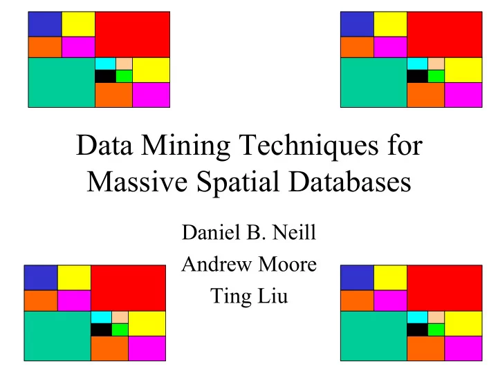
Data Mining Techniques for Massive Spatial Databases

Daniel B. Neill Andrew Moore Ting Liu

What is data mining?

• Finding relevant patterns in data
• Datasets are often huge and high-

dimensional, e.g. astrophysical sky survey

200 attributes: position (numeric), shape (categorical), spectra (complex structure), etc. 500 million galaxies and

• ther objects

Data is typically noisy, and some values may be missing

Query-based vs. pattern-based

Pattern Query (which patterns are we interested in finding?) Generality of query

“Give me the mean intensity of all galaxies in this part of the sky…” “Show me any individual objects with suprising attribute values…” “What’s interesting in this dataset?” “How do spiral galaxies differ from elliptical galaxies?” “Do spiral or elliptical galaxies typically have greater intensities?”

single query significance adjusting for covariates multiple queries distinguish real/spurious many possible queries what makes interesting? interesting groups

Difficulties in data mining

• Distingushing relevant patterns from those

due to chance and multiple testing

• Computation on massive data sets

– Each individual query may be very expensive: huge number of records, high dimensionality! – Typical data mining tasks require many queries!

Simple data mining approaches

• Exhaustive search
• Sampling
• Caching queries

Simple data mining approaches

• Exhaustive search
• Sampling
• Caching queries

“How many pairs of galaxies within distance d of each other?” Just count them! Problem:

• ften computationally infeasible

500 million data points 2.5 x 1017 pairs!

Simple data mining approaches

• Exhaustive search
• Sampling
• Caching queries

“How many pairs of galaxies within distance d of each other?” Sample 1 million pairs of galaxies, use to estimate… Problems:

• nly approximate answers to queries

may miss rare events can’t make fine distinctions

Simple data mining approaches

• Exhaustive search
• Sampling
• Caching queries

“How many pairs of galaxies within distance d of each other?” Precompute a histogram of the N2

• distances. Then each query d can be

answered quickly. Advantages: can reuse precomputed information, amortizing cost over many queries Problems: precomputation may be too expensive what to precompute?

Advanced data mining techniques

• More complex data structures faster queries.
• Grouped computation: simultaneous computation

for a group of records rather than for each record individually.

– What can be ruled out? – What can be ruled in? – Cache and use sufficient statistics (centroids, bounds…)

We focus here on some advanced techniques for mining of spatial data: answering queries about points or groups of points in space.

Space-partitioning trees!

Outline

• Introduction to space-partitioning trees

– What are they, and why would we want to use them? – Quadtrees and kd-trees

• Nearest neighbor with space-partitioning trees

– Ball trees

• Cluster detection with space-partitioning trees

– Overlap trees

Why space-partitioning trees?

• Many machine learning tasks involve searching

for points or regions in space.

– Clustering, regression, classification, correlation, density estimation…

• Space-partitioning trees can make our searches

tens to thousands of times faster!

– Particularly important for applications where we want to obtain information from massive datasets in real time: for example, monitoring for disease outbreaks.

Multi-resolution search

• Rather than examining each data point separately, we can

group the data points according to their position in space, then examine each group.

• Typically, some groups are more “interesting” than others:

– We may need to examine each individual point in group G… – Or we may need only summary information about G… – Or we might not even need to search G at all!

• How to group the points?

– A few large groups? – A lot of small groups?

Better idea: search different regions at different resolutions!

Multi-resolution search (2)

• Top-down search: start by looking at the “bird’s

eye view” (coarse resolution) then search at progressively finer resolutions as necessary.

Often, we can get enough information about most regions from the “bird’s eye view,” and only need to search a small subset of regions more closely!

Space partitioning in 1-D

• A binary tree can be thought of

as partitioning a 1-D space; this is the simplest space- partitioning tree!

• Point search: O(log N)
• Range search (find all pts in

[a,b]): O(M+log N) (0, 20) (0, 10) (10, 20) (0, 5) (5, 10) (10, 15) (15, 20) How can we extend this to multiple dimensions?

Quadtrees

• In a quadtree structure, each

parent region is split into four children (“quadrants”) along two iso-oriented lines; these can then be further split.

• To search a quadtree:

– start at the root (all of space) – recursively compare query (x,y) to split point (x’,y’), selecting

• ne of the four children based
• n these two comparisons.

Quadtrees (2)

• How to split a region into quadrants?
• Method 1: make all four quadrants equal.
• Method 2: split on points inserted into tree.
• Method 3: split on median in each dimension.

Method 1 Method 2 Method 3 What are the advantages and disadvantages of each method?

Extending quadtrees

• Quadtrees can be trivially extended to hold higher

dimensional data.

• In 3-D, we have an oct-tree

– splits space into eighths

• Problem #1: In d dimensions, we must split each

parent node into 2d children!

• Problem #2: To search a d-dimensional quadtree,

we must do d comparisons at each decision node.

• How can we do better?

kd-trees

• In a kd-tree, each parent is split

into two regions along a single iso-oriented line.

• Typically we cycle through the

dimensions (1st level splits on x, 2nd level on y, etc.).

• Again we can split into equal

halves, on inserted points, or on the median point.

• More flexible; can even do

different splits on different children, as shown here.

Note: even in d dimensions, a parent will have only two children.

Searching in kd-trees

• Can do point search in O(log

N) as in binary tree.

• Region search (i.e. search for

all points in d-dimensional interval): O(M+N(1-1/d))

• If xmin < xsplit, must search left

child; if xmax > xsplit, must search right child. Slower than 1-D region search because we might have to search both subregions!

Augmenting kd-trees

• In a standard kd-tree, all

information is stored in the leaves.

• We can make kd-trees much more

useful by augmenting them with summary information at each non- leaf node. For example:

– Number of data points in region – Bounding hyper-rectangle – Mean, covariance matrix, etc.

• Deng and Moore call these

“multiresolution kd-trees.” 5 2 3 1 1 3

A simple example: 2-point correlation

• How many pairs of points are

within radius r of each other?

• A statistical measure of the

“clumpiness” of a set of points.

• Naïve approach O(N2): consider

all pairs of points.

• Better approach: store points in

an mrkd-tree!

• This allows computation of the

2-point correlation in O(N3/2). 5 2 3 1 1 3

2-point correlation (2)

• For each point in the dataset, find

how many points are within radius r of the query point.

• To do so, we search the mrkd-

tree top-down, looking at the bounding rectangle of each node.

– If all within distance r, add number

• f points in node.

– If none within distance r, add 0. – If some within distance r:

• Recurse on each child.
• Add results together.

5 2 3 1 1 3

Dual-tree search

• Gray and Moore (2001) show

that 2-point correlation can be computed even faster by using two kd-trees, and traversing both simultaneously.

• Rather than doing a separate

search of the grouped data for each query point, we also group the query points using another kd-tree.

– 2x speedup vs. single tree.

5 2 3 1 1 3

Mo(o)re applications

• Deng and Moore (1995): mrkd-trees for kernel regression.
• Moore et al. (1997): mrkd-trees for locally weighted

polynomial regression.

• Moore (1999): mrkd-trees for EM-based clustering.
• Gray and Moore (2001-2003): dual-tree search for kernel

density estimation, N-point correlation, etc.

• STING (Wang et al., 1997): “statistical information grids”

(augmented quadtrees) for approximate clustering.

• Also used in many computational geometry applications

(e.g. storing geometric objects in “spatial databases”).

Nearest neighbor using space- partioning trees

(These slides adapted from work by Ting Liu and Andrew Moore)

A Set of Points in a metric space

To do nearest neighbor, we’ll use another kind of space-partitioning tree: the ball tree or metric tree.

Ball Tree root node

A Ball Tree

A Ball Tree

A Ball Tree

A Ball Tree

Ball-trees: properties

Let Q be any query point and let x be a point inside ball B |x-Q| ≥ |Q - B.center| - B.radius |x-Q| ≤ |Q - B.center| + B.radius

Q

B.center

x

Q

Goal: Find out the 2-nearest neighbors of Q.

Q

Start at the root

Q

Recurse down the tree

Q

Q

Q

Q

We’ve hit a leaf node, so we explicitly look at the points in the node

Q

Two nearest neighbors found so far are in pink (remember we have yet to search the blue circles)

Q

Now we don’t have to search any circle entirely outside the white circle

Q

Q

Q

Q

Q

Q

Q

Q

Q

Q

We’ve hit a leaf node, so we explicitly look at the points in the node

Q

We’ve found a new nearest neighbor, so we can shrink the white circle

Q

Q

Q

All done!

The punch line

• This method is much faster than exhaustive search

for finding the k nearest neighbors of a point.

• But in k-NN classification, we don’t actually need

to find the neighbors… just determine which class is most common among these neighbors!

• So much faster ball-tree algorithms are possible!

– See Liu, Moore, and Gray (NIPS 2003) for one such algorithm, using two ball trees (one for positive class,

• ne for negative class)

Cluster detection with space- partitioning trees

Daniel B. Neill Andrew W. Moore

What is a cluster?

• A spatial region where some

quantity (the count) is significantly higher than expected, given some underlying baseline.

• For example:

– count = number of disease cases in a region over some time period. – baseline = expected number of disease cases in that region

• ver that time period.

We found 30 respiratory cases in this region when we only expected 20. Is this significant?

What is a cluster?

We found 30 respiratory cases in this region when we only expected 20. Is this significant?

Significant increase: we believe that the increase results from different underlying distributions inside and outside the region. vs. Non-significant increase: we believe that the underlying distributions inside and

• utside the region are the same, and the

increase resulted from chance fluctuations.

Goals of cluster detection

• Identifying potential clusters

– Are there any clusters? If so, how many? – Location, shape, and size of each potential cluster.

• Determining whether each potential cluster

is likely to be a “true” cluster or a chance

• ccurrence.

– Statistical significance testing.

Application #1: outbreak detection

• Goal: early, automatic detection of disease epidemics.

– Responding to bioterrorist attacks (ex. anthrax). – Naturally occurring outbreaks (ex. SARS, hepatitis).

• There is often a significant time lag between exposure to a

pathogen and a definitive diagnosis. However, symptom

• nset typically precedes diagnosis by days or even weeks.
• Faster detection using syndromic data: we look for clusters
• f disease symptoms that indicate a potential outbreak.

– Emergency Dept. visits – 911 calls – OTC drug sales

Early detection can save lives!

The National Retail Data Monitor

• The National Retail Data Monitor (NRDM) receives data from 20,000 retail

stores (grocery stores, pharmacies, etc.) nationwide.

• Data: number of over the counter drugs sold daily, for each store, in each of 18

categories (e.g. cough and cold, anti-diarrheal, pediatric electrolytes)

• Given this data, we want to determine daily if any disease outbreaks are
• ccurring, and if so, identify the type, location, size, and severity of outbreaks.

A screen shot from NRDM For more details

• n NRDM, go to

www.rods.health.pitt.edu

Application #2: brain imaging

• Goal: discover regions of

brain activity corresponding to given cognitive tasks.

• Word recognition task:

Noun! Verb!

Application #2: brain imaging

• fMRI image:

– 3D picture of brain activity – Brain discretized into 64 x 64 x 14 grid of “voxels.” – Amount of “activation” in each voxel corresponds to brain activity in that region.

• We compare fMRI images

corresponding to different cognitive tasks, looking for clusters of increased brain activity.

Problem overview

• Assume data has been

aggregated to a d- dimensional grid of cells.

– d = 2 for epidemiology – d = 3 for fMRI – More dimensions can be used if we want to take time, covariates, etc. into account.

• Each grid cell si has a count

ci and a baseline bi.

B=5000 C=27 B=3500 C=14 B=4500 C=22 B=3000 C=15 B=1000 C=5 B=5000 C=26 B=4000 C=17 B=3000 C=12 B=2000 C=12 B=1000 C=4 B=5000 C=19 B=5000 C=25 B=4000 C=43 B=3000 C=37 B=4000 C=20 B=4800 C=18 B=4800 C=20 B=4000 C=40 B=3000 C=22 B=4000 C=16 B=4700 C=20 B=3000 C=13 B=3000 C=18 B=2000 C=20 B=1000 C=4

Baseline of cell Count of cell This is a significant cluster.

Application domains

• In epidemiology:

– Counts ci represent number of disease cases in a region, or some related observable quantity (e.g. Emergency Department visits, sales

• f OTC medications).

– Baselines bi can be populations

• btained from census data, or

expected counts obtained from historical data (e.g. past OTC sales).

• In brain imaging:

– Counts ci represent fMRI activation in a given voxel under some experimental condition. – Baselines bi represent fMRI activation under null condition.

Application domains

• In both domains:

– Goal is to find spatial regions where the counts ci are significantly higher than expected, given the baselines bi. – “Higher than expected” requires an underlying model of what we expect!

• If there are no clusters…
• If clusters are present…

Problem overview

• To detect clusters:

– Find the most significant spatial regions. – Calculate statistical significance of these regions.

• We focus here on finding

the single most significant region S* (and its p-value).

– If p-value > α, no significant clusters exist. – If p-value < α, then S* is significant; we can then examine secondary clusters.

B=5000 C=27 B=3500 C=14 B=4500 C=22 B=3000 C=15 B=1000 C=5 B=5000 C=26 B=4000 C=17 B=3000 C=12 B=2000 C=12 B=1000 C=4 B=5000 C=19 B=5000 C=25 B=4000 C=43 B=3000 C=37 B=4000 C=20 B=4800 C=18 B=4800 C=20 B=4000 C=40 B=3000 C=22 B=4000 C=16 B=4700 C=20 B=3000 C=13 B=3000 C=18 B=2000 C=20 B=1000 C=4

Which regions to search?

• We choose to search over the

space of all rectangular regions.

• We typically expect clusters to

be convex; thus inner/outer bounding boxes are reasonably close approximations to shape.

• We can find clusters with high

aspect ratios.

– Important in epidemiology since disease clusters are often elongated (e.g. from windborne pathogens). – Important in brain imaging because of the brain’s “folded sheet” structure.

Which regions to search?

• We choose to search over the

space of all rectangular regions.

• We typically expect clusters to

be convex; thus inner/outer bounding boxes are reasonably close approximations to shape.

• We can find clusters with high

aspect ratios.

– Important in epidemiology since disease clusters are often elongated (e.g. from windborne pathogens). – Important in brain imaging because of the brain’s “folded sheet” structure.

We can find non- axis-aligned rectangles by examining multiple rotations of the data.

Calculating significance

• Define models:

– of the null hypothesis H0: no clusters. – of the alternative hypotheses H1(S): clustering in region S.

• Derive a score function D(S) = D(C, B).

– Likelihood ratio: – To find the most significant region:

) | Data ( )) ( | Data ( ) (

1

H L S H L S D =

) ( max arg * S D S

S

=

Example: Kulldorff’s model

• Kulldorff’s spatial scan statistic is

commonly used by epidemiologists to detect disease clusters.

• Model: each count ci is generated from

a Poisson distribution with mean qbi.

– Count ci represents number of cases. – Baseline bi represents the at-risk population. – q represents the disease rate.

• This statistic is most powerful for

finding a single region of elevated disease rate (qin > qout).

qin = .02 qout = .01

Randomization testing

• Multiple hypothesis testing is a

major problem: over 1 billion regions for a 256 x 256 grid.

• To deal with this problem, we

must use randomization testing.

– Randomly create a large number

• f replica grids.

– Find the maximum D(S) for each replica, compare to the

• riginal region.

– p-value = proportion of replicas beating original. – The original region is significant if very few replicas have a higher D(S).

Summary of spatial scan framework

• 1. Calculate score function D(S) from model

(H0, H1(S)) using likelihood ratio.

• 2. Compute D(S) for all spatial regions S.
• 3. Return the region S* with highest D(S).
• 4. Compute p-value of S* by randomization

testing.

• 5. If S* is significant, find secondary

clusters.

The catch

Computing D(S) for all spatial regions S is expensive, since there are O(N4) rectangular regions for an NxN grid. Worse, randomization testing requires us to do the same O(N4) search for each replica grid, multiplying the runtime by the number of replicas. For a 256 x 256 grid, with 1000 replications: 1.1 trillion regions to search, which would take 14-45 days. This is far too slow for real-time cluster detection!

This is our motivation for a fast spatial scan!

How to speed up our search?

• How can we find the best

rectangular region without searching over every single rectangle?

• Use a space-partitioning tree?

– Problem: many subregions of a region are not contained entirely in either “child,” but overlap partially with each. kd-tree

How to speed up our search?

• How can we find the best

rectangular region without searching over every single rectangle?

• Use a space-partitioning tree?

– Problem: many subregions of a region are not contained entirely in either “child,” but overlap partially with each. kd-tree

The solution: Overlap-multiresolution partitioning

• We propose a partitioning approach in which

adjacent regions are allowed to partially overlap.

• The basic idea is to:

– Divide the grid into overlapping regions. – Bound the maximum score of subregions contained in each region. – Prune regions which cannot contain the most significant region. – Find the same region and p-value as the exhaustive approach… but hundreds or thousands of times faster!

S_3 S_1

S

S_C

some S_i, i = 1..4, Any subregion of S:

S_2 S_4

either a) is contained in

• r b) contains S_C.
• Parent region S is divided into four
• verlapping child regions: “left child” S1,

“right child” S2, “top child” S3, and “bottom child” S4.

• Then for any rectangular subregion S’ of

S, exactly one of the following is true:

– S’ is contained entirely in (at least) one of the children S1… S4. – S’ contains the center region SC, which is common to all four children.

• Starting with the entire grid G and

repeating this partitioning recursively, we

• btain the overlap-kd tree structure.

Overlap-multires partitioning

The overlap-kd tree (first two levels)

SC

d-dimensional partitioning

• Parent region S is divided into 2d
• verlapping children: an “upper child” and

a “lower child” in each dimension.

• Then for any rectangular subregion S’ of

S, exactly one of the following is true:

– S’ is contained entirely in (at least) one of the children S1… S2d. – S’ contains the center region SC, which is common to all the children.

• Starting with the entire grid G and

repeating this partitioning recursively, we

• btain the overlap-kd tree structure.

S5 S1 S2 S3 S4 S6 S

Properties of the overlap-kd tree

• Every rectangular region S’ in G is either:

– a gridded region (i.e. contained in the overlap-kd tree) – or an outer region of a unique gridded region S (i.e. S’ is contained in S and contains its center SC).

Overlap-multires partitioning

• The basic (exhaustive) algorithm: to

search a region S, recursively search S1… S2d, then search over all outer regions containing SC.

• We can improve the basic algorithm

by pruning: since all the outer regions

• f S contain the (large) center region

SC, we can calculate tight bounds on the maximum score, often allowing us not to search any of them.

S_3 S_1

S

S_C

some S_i, i = 1..4, Any subregion of S:

S_2 S_4

either a) is contained in

• r b) contains S_C.

Region pruning

• In our top-down search, we keep track of the best region

S* found so far, and its score D(S*).

• When we search a region S, we compute upper bounds on

the scores:

– Of all subregions S’ of S. – Of all outer subregions S’ (subregions of S containing SC).

• If the upper bounds for a region are worse than the best

score so far, we can prune.

– If no subregion can be optimal, prune completely (don’t search any subregions). – If no outer subregion can be optimal, recursively search the child regions, but do not search the outer regions. – If neither case applies, we must recursively search the children and also search over the outer regions.

Summary of results

• The fast spatial scan results in

huge speedups (as compared to exhaustive search), making fast real-time detection of clusters feasible.

• No loss of accuracy: fast spatial

scan finds the exact same regions and p-values as exhaustive search.

ED dataset

Results: ED dataset

• Western Pennsylvania Emergency

Department Data (256 x 256 grid):

– Our method: 21 minutes. – Exhaustive approach: 14 days! – ~1000x speedup.

• 10-20x faster than current state of the

art (Kulldorff’s SaTScan software).

• Using age, gender as covariates (and

thus searching a 4D grid): 235-325x speedups.

– Allows us to detect epidemics which have larger impact on specific demographics (e.g. elderly males, infants). ED dataset

Results: OTC, fMRI

• OTC data (256 x 256 grid):

– Our method: 47 minutes. – Exhaustive approach: 14 days! – ~400x speedups.

• Spatio-temporal cluster detection on

OTC (3D grid): 48-1400x speedups.

– Allows us to detect outbreaks that emerge more slowly (over multiple days).

• fMRI data (64 x 64 x 14 grid):

– 7-148x speedups as compared to exhaustive search approach. fMRI data from noun/verb word recognition task OTC data from National Retail Data Monitor

Case studies

• Rapidly finding clusters is all well and good… but are we

finding useful clusters?

• Best test: put system in practice, see what clusters it detects.
• Our system is currently running daily on OTC data.
• Some success stories:

– From OTC data, picked up an outbreak of cough-and-cold type symptoms resulting from the forest fires in California. – Using fMRI data, we were able to distinguish subjects performing the word recognition task from a control group (subjects fixating on a cursor); subjects doing word recognition had clusters of activity in visual cortex, Broca’s area, Wernicke’s area. More work still needs to be done in order to consistently detect useful clusters!

What you should know

• What is data mining, and why is it hard?
• Why space-partitioning trees are useful for

mining massive spatial datasets.

• How and when to use different types of

space-partitioning trees (quadtrees, kd-trees, mrkd-trees, ball trees, overlap trees…)