Data Mining and Matrices 03 Singular Value Decomposition Rainer - PowerPoint PPT Presentation
Data Mining and Matrices 03 Singular Value Decomposition Rainer Gemulla, Pauli Miettinen April 25, 2013 The SVD is the Swiss Army knife of matrix decompositions Diane OLeary, 2006 2 / 35 Outline The Definition 1 Properties of the
Data Mining and Matrices 03 – Singular Value Decomposition Rainer Gemulla, Pauli Miettinen April 25, 2013
The SVD is the Swiss Army knife of matrix decompositions —Diane O’Leary, 2006 2 / 35
Outline The Definition 1 Properties of the SVD 2 Interpreting SVD 3 SVD and Data Analysis 4 How many factors? Using SVD: Data processing and visualization Computing the SVD 5 Wrap-Up 6 About the assignments 7 3 / 35
The definition Theorem. For every A ∈ R m × n there exists m × m orthogonal matrix U and n × n orthogonal matrix V such that U T AV is an m × n diagonal matrix Σ that has values σ 1 ≥ σ 2 ≥ . . . ≥ σ min { n , m } ≥ 0 in its diagonal. I.e. every A has decomposition A = U Σ V T ◮ The singular value decomposition (SVD) The values σ i are the singular values of A Columns of U are the left singular vectors and columns of V the right singular vectors of A = T A U Σ V 4 / 35
Outline The Definition 1 Properties of the SVD 2 Interpreting SVD 3 SVD and Data Analysis 4 How many factors? Using SVD: Data processing and visualization Computing the SVD 5 Wrap-Up 6 About the assignments 7 5 / 35
The fundamental theorem of linear algebra The fundamental theorem of linear algebra states that every matrix A ∈ R m × n induces four fundamental subspaces: The range of dimension rank( A ) = r ◮ The set of all possible linear combinations of columns of A The kernel of dimension n − r ◮ The set of all vectors x ∈ R n for which Ax = 0 The coimage of dimension r The cokernel of dimension m − r The bases for these subspaces can be obtained from the SVD: Range: the first r columns of U Kernel: the last ( n − r ) columns of V Coimage: the first r columns of V Cokernel: the last ( m − r ) columns of U 6 / 35
Pseudo-inverses Problem. Given A ∈ R m × n and b ∈ R m , find x ∈ R n minimizing � Ax − b � 2 . If A is invertible, the solution is A − 1 Ax = A − 1 b ⇔ x = A − 1 b A pseudo-inverse A + captures some properties of the inverse A − 1 The Moose–Penrose pseudo-inverse of A is a matrix A + satisfying the following criteria (but it is possible that AA + � = I ) AA + A = A ◮ ◮ A + AA + = A + (cf. above) ◮ ( AA + ) T = AA T ( AA + is symmetric) ◮ ( A + A ) T = A + A (as is A + A ) If A = U Σ V T is the SVD of A , then A + = V Σ − 1 U T ◮ Σ − 1 replaces σ i ’s with 1 /σ i and transposes the result Theorem. The optimum solution for the above problem can be obtained using x = A + b . 7 / 35
Truncated (thin) SVD The rank of the matrix is the number of its non-zero singular values ◮ Easy to see by writing A = � min { n , m } σ i u i v T i =1 i The truncated (or thin) SVD only takes the first k columns of U and V and the main k × k submatrix of Σ ◮ A k = � k i = U k Σ k V T i =1 σ i u i v T k ◮ rank( A k ) = k (if σ k > 0) ◮ U k and V k are no more orthogonal, but they are column-orthogonal The truncated SVD gives a low-rank approximation of A T A U Σ V ≈ 8 / 35
SVD and matrix norms Let A = U Σ V T be the SVD of A . Then F = � min { n , m } � A � 2 σ 2 i =1 i � A � 2 = σ 1 ◮ Remember: σ 1 ≥ σ 2 ≥ · · · ≥ σ min { n , m } ≥ 0 Therefore � A � 2 ≤ � A � F ≤ √ n � A � 2 F = � k The Frobenius of the truncated SVD is � A k � 2 i =1 σ 2 i F = � min { n , m } ◮ And the Frobenius of the difference is � A − A k � 2 σ 2 i = k +1 i The Eckart–Young theorem Let A k be the rank- k truncated SVD of A . Then A k is the closest rank- k matrix of A in the Frobenius sense. That is � A − A k � F ≤ � A − B � F for all rank- k matrices B . 9 / 35
Eigendecompositions An eigenvector of a square matrix A is a vector v such that A only changes the magnitude of v ◮ I.e. Av = λ v for some λ ∈ R ◮ Such λ is an eigenvalue of A The eigendecomposition of A is A = Q ∆ Q − 1 ◮ The columns of Q are the eigenvectors of A ◮ Matrix ∆ is a diagonal matrix with the eigenvalues Not every (square) matrix has eigendecomposition ◮ If A is of form BB T , it always has eigendecomposition The SVD of A is closely related to the eigendecompositions of AA T and A T A ◮ The left singular vectors are the eigenvectors of AA T ◮ The right singular vectors are the eigenvectors of A T A ◮ The singular values are the square roots of the eigenvalues of both AA T and A T A 10 / 35
Outline The Definition 1 Properties of the SVD 2 Interpreting SVD 3 SVD and Data Analysis 4 How many factors? Using SVD: Data processing and visualization Computing the SVD 5 Wrap-Up 6 About the assignments 7 11 / 35
Factor interpretation The most common way to interpret SVD is to consider the columns of U (or V ) ◮ Let A be objects-by-attributes and U Σ V T its SVD ◮ If two columns have similar values in a row of V T , these attributes are somehow similar (have strong correlation) ◮ If two rows have similar values in a column of U , these users are somehow similar Example: people’s ratings of − 0.4 different wines − 0.3 Scatterplot of first and − 0.2 second column of U − 0.1 ◮ left: likes wine U2 0 ◮ right: doesn’t like ◮ up: likes red wine 0.1 ◮ bottom: likes white vine 0.2 Conclusion: winelovers like 0.3 0.25 0.2 0.15 0.1 0.05 0 − 0.05 − 0.1 − 0.15 − 0.2 − 0.25 U1 red and white, others care Figure 3.2. The first two factors for a dataset ranking wines. more 12 / 35 Skillicorn, p. 55
Geometric interpretation Let U Σ V T be the SVD of M SVD shows that every linear mapping y = Mx can be considered as a series of rotation, stretching, and rotation operations ◮ Matrix V T performs the first rotation y 1 = V T x ◮ Matrix Σ performs the stretching y 2 = Σ y 1 ◮ Matrix U performs the second rotation y = Uy 2 13 / 35 Wikipedia user Georg-Johann
Dimension of largest variance The singular vectors give the dimensions of the variance in the data X 3 ◮ The first singular vector is the dimension of the largest variance ◮ The second singular vector is the orthogonal dimension of the second X 1 X 2 largest variance ⋆ First two dimensions span a hyperplane u 2 From Eckart–Young we know that if we project the data to the spanned hyperplanes, the distance of the u 1 projection is minimized (a) Optimal 2D Basis 14 / 35 Zaki & Meira Fundamentals of Data Mining Algorithms , manuscript 2013
Component interpretation Recall that we can write A = U Σ V T = � r i = � r i =1 σ i u i v T i =1 A i ◮ A i = σ i v i u T i This explains the data as a sums of (rank-1) layers ◮ The first layer explains the most ◮ The second corrects that by adding and removing smaller values ◮ The third corrects that by adding and removing even smaller values ◮ . . . The layers don’t have to be very intuitive 15 / 35
Outline The Definition 1 Properties of the SVD 2 Interpreting SVD 3 SVD and Data Analysis 4 How many factors? Using SVD: Data processing and visualization Computing the SVD 5 Wrap-Up 6 About the assignments 7 16 / 35
Outline The Definition 1 Properties of the SVD 2 Interpreting SVD 3 SVD and Data Analysis 4 How many factors? Using SVD: Data processing and visualization Computing the SVD 5 Wrap-Up 6 About the assignments 7 17 / 35
Problem Most data mining applications do not use full SVD, but truncated SVD ◮ To concentrate on “the most important parts” But how to select the rank k of the truncated SVD? ◮ What is important, what is unimportant? ◮ What is structure, what is noise? ◮ Too small rank: all subtlety is lost ◮ Too big rank: all smoothing is lost Typical methods rely on singular values in a way or another 18 / 35
Guttman–Kaiser criterion and captured energy Perhaps the oldest method is the Guttman–Kaiser criterion: ◮ Select k so that for all i > k , σ i < 1 ◮ Motivation: all components with singular value less than unit are uninteresting Another common method is to select enough singular values such that the sum of their squares is 90% of the total sum of the squared singular values ◮ The exact percentage can be different (80%, 95%) ◮ Motivation: The resulting matrix “explains” 90% of the Frobenius norm of the matrix (a.k.a. energy) Problem: Both of these methods are based on arbitrary thresholds and do not consider the “shape” of the data 19 / 35
Cattell’s Scree test The scree plot plots the singular values in decreasing order ◮ The plot looks like a side of the hill, thence the name The scree test is a subjective decision on the rank based on the shape of the scree plot The rank should be set to a point where ◮ there is a clear drop in the magnitudes of the singular values; or ◮ the singular values start to even out Problem: Scree test is subjective, and many data don’t have any clear shapes to use (or have many) ◮ Automated methods have been developed to detect the shapes from the scree plot 90 20 18 80 16 70 14 60 12 50 10 40 8 30 6 20 4 10 2 0 0 0 10 20 30 40 50 60 70 80 90 100 0 10 20 30 40 50 60 70 80 90 100 20 / 35
Recommend
More recommend
Explore More Topics
Stay informed with curated content and fresh updates.
