Data Mining and Machine Learning: Fundamental Concepts and - PowerPoint PPT Presentation

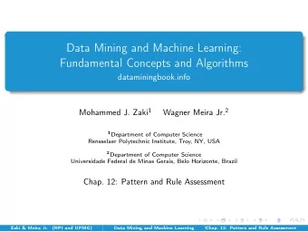
Data Mining and Machine Learning: Fundamental Concepts and Algorithms dataminingbook.info Mohammed J. Zaki 1 Wagner Meira Jr. 2 1 Department of Computer Science Rensselaer Polytechnic Institute, Troy, NY, USA 2 Department of Computer Science Universidade Federal de Minas Gerais, Belo Horizonte, Brazil Chapter 2: Numeric Attributes Zaki & Meira Jr. (RPI and UFMG) Data Mining and Machine Learning Chapter 2: Numeric Attributes 1 / 35

Univariate Analysis Univariate analysis focuses on a single attribute at a time. The data matrix D is an n × 1 matrix,   X   x 1     x 2 D =     . .   . x n where X is the numeric attribute of interest, with x i ∈ R . X is assumed to be a random variable, and the observed data a random sample drawn from X , i.e., x i ’s are independent and identically distributed as X . In the vector view, we treat the sample as an n -dimensional vector, and write X ∈ R n . Zaki & Meira Jr. (RPI and UFMG) Data Mining and Machine Learning Chapter 2: Numeric Attributes 2 / 35

Empirical Probability Mass Function The empirical probability mass function (PMF) of X is given as � n f ( x ) = P ( X = x ) = 1 ˆ I ( x i = x ) n i = 1 where the indicator variable I takes on the value 1 when its argument is true, and 0 otherwise. The empirical PMF puts a probability mass of 1 n at each point x i . The empirical cumulative distribution function (CDF) of X is given as � n F ( x ) = 1 ˆ I ( x i ≤ x ) n i = 1 The inverse cumulative distribution function or quantile function for X is defined as follows: F − 1 ( q ) = min { x | ˆ F ( x ) ≥ q } for q ∈ [ 0 , 1 ] The inverse CDF gives the least value of X , for which q fraction of the values are higher, and 1 − q fraction of the values are lower. Zaki & Meira Jr. (RPI and UFMG) Data Mining and Machine Learning Chapter 2: Numeric Attributes 3 / 35

Mean The mean or expected value of a random variable X is the arithmetic average of the values of X . It provides a one-number summary of the location or central tendency for the distribution of X . If X is discrete, it is defined as � µ = E [ X ] = x · f ( x ) x where f ( x ) is the probability mass function of X . If X is continuous it is defined as � ∞ µ = E [ X ] = x · f ( x ) dx −∞ where f ( x ) is the probability density function of X . Zaki & Meira Jr. (RPI and UFMG) Data Mining and Machine Learning Chapter 2: Numeric Attributes 4 / 35

Sample Mean The sample mean is a statistic, that is, a function ˆ µ : { x 1 , x 2 ,..., x n } → R , defined as the average value of x i ’s: � n µ = 1 ˆ x i n i = 1 It serves as an estimator for the unknown mean value µ of X . An estimator ˆ θ is called an unbiased estimator for parameter θ if E [ˆ θ ] = θ for every possible value of θ . The sample mean ˆ µ is an unbiased estimator for the population mean µ , as � � � n � n � n 1 = 1 E [ x i ] = 1 E [ˆ µ ] = E x i µ = µ n n n i = 1 i = 1 i = 1 We say that a statistic is robust if it is not affected by extreme values (such as outliers) in the data. The sample mean is not robust because a single large value can skew the average. Zaki & Meira Jr. (RPI and UFMG) Data Mining and Machine Learning Chapter 2: Numeric Attributes 5 / 35

bC bC bC bC bC bC bC bC bC bC bC bC bC bC bC bC bC bC bC bC bC bC bC bC bC bC bC bC bC bC bC bC bC bC bC bC bC bC bC bC bC bC bC bC bC bC bC bC bC bC bC bC bC bC bC bC bC bC bC bC bC bC bC bC bC bC bC bC bC bC bC bC bC bC bC bC bC bC bC bC bC bC bC bC bC bC bC bC bC bC bC bC bC bC bC bC bC b bC bC bC bC bC bC bC bC bC bC bC bC bC bC bC bC bC bC bC bC bC bC bC bC bC bC bC bC bC bC bC bC bC bC bC bC bC bC bC bC bC bC bC bC bC bC bC bC bC bC bC bC bC Sample Mean: Iris sepal length Frequency X 1 4 4 . 5 5 . 0 5 . 5 6 . 0 6 . 5 7 . 0 7 . 5 8 . 0 ˆ µ = 5 . 843 Zaki & Meira Jr. (RPI and UFMG) Data Mining and Machine Learning Chapter 2: Numeric Attributes 6 / 35

Median The median of a random variable is defined as the value m such that P ( X ≤ m ) ≥ 1 2 and P ( X ≥ m ) ≥ 1 2 The median m is the “middle-most” value; half of the values of X are less and half of the values of X are more than m . In terms of the (inverse) cumulative distribution function, the median is the value m for which F ( m ) = 0 . 5 or m = F − 1 ( 0 . 5 ) The sample median is given as F ( m ) = 0 . 5 or m = ˆ ˆ F − 1 ( 0 . 5 ) Median is robust, as it is not affected very much by extreme values. Zaki & Meira Jr. (RPI and UFMG) Data Mining and Machine Learning Chapter 2: Numeric Attributes 7 / 35

Mode The mode of a random variable X is the value at which the probability mass function or the probability density function attains its maximum value, depending on whether X is discrete or continuous, respectively. The sample mode is a value for which the empirical probability mass function attains its maximum, given as ˆ mode ( X ) = argmax f ( x ) x Zaki & Meira Jr. (RPI and UFMG) Data Mining and Machine Learning Chapter 2: Numeric Attributes 8 / 35

Empirical CDF: sepal length 1 . 00 0 . 75 F ( x ) 0 . 50 ˆ 0 . 25 0 4 4 . 5 5 . 0 5 . 5 6 . 0 6 . 5 7 . 0 7 . 5 8 . 0 x Zaki & Meira Jr. (RPI and UFMG) Data Mining and Machine Learning Chapter 2: Numeric Attributes 9 / 35

Empirical Inverse CDF: sepal length 8 . 0 7 . 5 7 . 0 6 . 5 F − 1 ( q ) 6 . 0 ˆ 5 . 5 5 . 0 4 . 5 4 0 0 . 25 0 . 50 0 . 75 1 . 00 q The median is 5 . 8, since F ( 5 . 8 ) = 0 . 5 or 5 . 8 = ˆ ˆ F − 1 ( 0 . 5 ) Zaki & Meira Jr. (RPI and UFMG) Data Mining and Machine Learning Chapter 2: Numeric Attributes 10 / 35

Range The value range or simply range of a random variable X is the difference between the maximum and minimum values of X , given as r = max { X } − min { X } The sample range is a statistic, given as n n ˆ r = max i = 1 { x i } − min i = 1 { x i } Range is sensitive to extreme values, and thus is not robust. A more robust measure of the dispersion of X is the interquartile range (IQR) , defined as IQR = F − 1 ( 0 . 75 ) − F − 1 ( 0 . 25 ) The sample IQR is given as IQR = ˆ � F − 1 ( 0 . 75 ) − ˆ F − 1 ( 0 . 25 ) Zaki & Meira Jr. (RPI and UFMG) Data Mining and Machine Learning Chapter 2: Numeric Attributes 11 / 35

Variance and Standard Deviation The variance of a random variable X provides a measure of how much the values of X deviate from the mean or expected value of X �  ( x − µ ) 2 f ( x )  if X is discrete    � ( X − µ ) 2 � x σ 2 = var( X ) = E = � ∞    ( x − µ ) 2 f ( x ) dx  if X is continuous −∞ The standard deviation σ , is the positive square root of the variance, σ 2 . The sample variance is defined as � n σ 2 = 1 µ ) 2 ˆ ( x i − ˆ n i = 1 and the sample standard deviation is � � � n � � 1 µ ) 2 ˆ σ = ( x i − ˆ n i = 1 Zaki & Meira Jr. (RPI and UFMG) Data Mining and Machine Learning Chapter 2: Numeric Attributes 12 / 35

Geometric Interpretation of Sample Variance The sample values for X comprise a vector in n -dimensional space, where n is the sample size. Let Z denote the centered sample   x 1 − ˆ µ   x 2 − ˆ µ   Z = X − 1 · ˆ µ =   . .   . x n − ˆ µ where 1 ∈ R n is the vector of ones. Sample variance is squared magnitude of the centered attribute vector, normalized by the sample size: � n σ 2 = 1 n � Z � 2 = 1 n Z T Z = 1 µ ) 2 ˆ ( x i − ˆ n i = 1 Zaki & Meira Jr. (RPI and UFMG) Data Mining and Machine Learning Chapter 2: Numeric Attributes 13 / 35

Variance of the Sample Mean and Bias Sample mean ˆ µ is itself a statistic. We can compute its mean value and variance E [ˆ µ ] = µ µ − µ ) 2 ] = σ 2 var (ˆ µ ) = E [(ˆ n The sample mean ˆ µ varies or deviates from the mean µ in proportion to the population variance σ 2 . However, the deviation can be made smaller by considering larger sample size n . The sample variance is a biased estimator for the true population variance, since � n − 1 � σ 2 ] = σ 2 E [ˆ n But it is asymptotically unbiased, since σ 2 ] → σ 2 E [ˆ as n → ∞ Zaki & Meira Jr. (RPI and UFMG) Data Mining and Machine Learning Chapter 2: Numeric Attributes 14 / 35

Bivariate Analysis In bivariate analysis, we consider two attributes at the same time. The data D comprises an n × 2 matrix:   X 1 X 2   x 11 x 12     x 21 x 22 D =     . . . .   . . x n 1 x n 2 Geometrically, D comprises n points or vectors in 2-dimensional space x i = ( x i 1 , x i 2 ) T ∈ R 2 D can also be viewed as two points or vectors in an n -dimensional space: X 1 = ( x 11 , x 21 ,..., x n 1 ) T X 2 = ( x 12 , x 22 ,..., x n 2 ) T In the probabilistic view, X = ( X 1 , X 2 ) T is a bivariate vector random variable, and the points x i (1 ≤ i ≤ n ) are a random sample drawn from X , that is, x i ’s IID with X . Zaki & Meira Jr. (RPI and UFMG) Data Mining and Machine Learning Chapter 2: Numeric Attributes 15 / 35