Data Assimilation for Stochastic Transport Models Dan Crisan - PowerPoint PPT Presentation

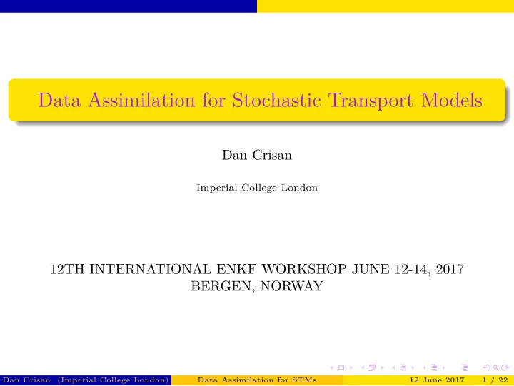
. . . . . . . . . . . . . . Data Assimilation for Stochastic Transport Models Dan Crisan Imperial College London 12TH INTERNATIONAL ENKF WORKSHOP JUNE 12-14, 2017 BERGEN, NORWAY Dan Crisan (Imperial College London) Data Assimilation for STMs 12 June 2017 . . . . . . . . . . . . . . . . . . . . . . . . . . 1 / 22

. . . . . . . . . . . . . . Talk Synopsis What is Data Assimilation ? What is Stochastic Filtering ? Why is the high-dimensional problem hard ? Stochastic transport models Data assimilation for STMs Dan Crisan (Imperial College London) Data Assimilation for STMs 12 June 2017 . . . . . . . . . . . . . . . . . . . . . . . . . . . 2 / 22 Data Assimilation ⇔ Stochastic Filtering: a dictionary.

. Mathematics of Connecting Dynamical Systems to Data, MFO” . . . . . . . . . What is DA ? What is data assimilation ? Jana de Wiljes, Sebastian Reich, Andrew Stuart ”Data Assimilation: The The seamless integration of large data sets into computational models provides . one of the central challenges for the mathematical sciences of the 21st century. When the computational model is based on dynamical systems and the data is time ordered, the process of combining data and models is called data assimilation. Mark Asch, Marc Bocquet, Ma฀lle Nodet, “Data Assimilation: Methods, Algorithms, and Applications” Data assimilation is an approach that combines observations and model output, with the objective of improving the latter. Dan Crisan (Imperial College London) Data Assimilation for STMs 12 June 2017 . . . . . . . . . . . . . . . . . . . . . . . . . . . . . . 3 / 22

. numerical model with new information about that system in the form of . . . . . . . . What is DA ? Peter Jan van Leeuwen, ”Nonlinear Data Assimilation for high-dimensional systems ฀with geophysical applications. Data assimilation combines past knowledge of a system in the form of a observations of that system. . Sebastian Reich, Colin Cotter, “Probabilistic Forecasting and Bayesian Data Assimilation” Data assimilation was coined in the computational geoscience community to describe methodologies for improving forecasting skill by combining measured data with computer generated forecasts. More specifjcally, data assimilation algorithms meld computational models with sets of observations in order to, for example, reduce uncertainties in the model forecasts or to adjust model parameters. Dan Crisan (Imperial College London) Data Assimilation for STMs 12 June 2017 . . . . . . . . . . . . . . . . . . . . . . . . . . . . . . . 4 / 22

. . . . . . . . . . . . . . . What is stochastic fjltering ? Stochastic fjltering The process of using partial observations and a stochastic model to make inferences about an evolving dynamical system. Courtesy of Oana Lang (Imperial College London) Dan Crisan (Imperial College London) Data Assimilation for STMs 12 June 2017 . . . . . . . . . . . . . . . . . . . . . . . . . . 5 / 22

. . . . . . . . . . . . . . The Filtering Problem Framework: discrete/continuous time X the signal process - “hidden component” Y the observation process - “the data” Discrete framework: Continuous framework: Dan Crisan (Imperial College London) Data Assimilation for STMs 12 June 2017 . . . . . . . . . . . . . . . . . . . . . . . 6 / 22 . . . The fjltering problem: Find the conditional distribution of the signal X t given Y t = σ ( Y s , s ∈ [ 0 , t ]) , i.e., π t ( A ) = P ( X t ∈ A |Y t ) , t ≥ 0 , A ∈ B ( R d ) . { X t } t ≥ 0 Markov chain P ( X t ∈ dx t | X t − 1 = x t − 1 ) = f t ( x t | x t − 1 ) dt , { X t , Y t } t ≥ 0 P ( Y t ∈ dy | X t = x t ) = g t ( y | x t ) dy dX t = f ( X t ) dt + σ ( X t ) dV t , dY t = h ( X t ) dt + dW t .

. Gaussian . mean weight position weight approximations approximations j particle problem should contain three parts: The description of a numerical approximation for the solution of the fjltering How do we defjne an approximation ? The Filtering Problem . j covariance matrix . forecast 12 June 2017 Data Assimilation for STMs (Imperial College London) Dan Crisan 3. The measure of the approximating error: assimilation t 2. The law of evolution of the approximation: selection mutation t approximations Gaussian approximations particle . 7 / 22 . . . . . . . . . . . . . . . . . . . . . . . . . . . . . . . . . . . ( a j ( t ) , v 1 j ( t ) , . . . , v d j ( t ) ) n ( a j ( t ) , v 1 j ( t ) , . . . , v d j ( t ) , ω 11 ( t ) , . . . , ω dd ( t ) ) n j = 1 j = 1 � �� � � �� � � �� � � �� � � �� � t = ∑ n t = ∑ n π t � π n j = 1 a j ( t ) δ v j ( t ) π t � π n j = 1 a j ( t ) N ( v j ( t ) , ω j ( t )) ���� ���� ���� ���� − → − → − → − → π n model ¯ π n π n π n model ¯ π n π n t + δ t + δ t + δ t + δ { Y s } s ∈ [ t , t + δ ] { Y s } s ∈ [ t , t + δ ] sup E [ | π n t ( φ ) − π t ( φ ) | ] , π t − ˆ ˆ π n t , ∥ π n t − π t ∥ TV . ϕ ∈ C b

. . . . . . . . . . . . The Filtering Problem . Quantized information = particles The quantized information is modelled by n stochastic processes Generalized particle fjlters: classical particle fjlters gaussian approximations wavelets grid methods Dan Crisan (Imperial College London) Data Assimilation for STMs 12 June 2017 . . . . . . . . . . . . . . . 8 / 22 . . . . . . . . . . . . { p i ( t ) , t > 0 } i = 1 , ..., n , p i ( t ) ∈ R N . We think of the processes p i as the trajectories of n (generalized) particles. Typically N > d, where d is the dimension of the state space. π n t = Λ n t ( p i ( t ) , t > 0 i = 1 , ..., n ) .

. The Filtering Problem . . . . . . . . . . The classical particle fjlter . The classical/standard/bootstrap/garden-variety particle fjlter sequence of a system of weighted particles n 1 i n a n Dan Crisan (Imperial College London) Data Assimilation for STMs 12 June 2017 . . . . . . . . . . . . . . . 9 / 22 . . . . . . . . . . . . . π n = { π n ( t ) , t ≥ 0 } the occupation measure/empirical distribution of a ∑ ∑ π n ( 0 ) = n δ x n − → π n ( t ) = ¯ i ( t ) δ V n i ( t ) . i = 1 i = 1

. . . . . . . . . . . . . . . The Filtering Problem The classical particle fjlter Courtesy of Oana Lang (Imperial College London) Theorem Dan Crisan (Imperial College London) Data Assimilation for STMs 12 June 2017 . . . . . . . . . . . . . . . . . . . . 10 / 22 . . . . . π n converges to π . Moreover t ( φ ) − π t ( φ ) ∥ p ≤ α ( T , p ) ∥ π n √ n sup sup . t ∈ [ 0 , T ] { ϕ ∈ C 1 b ( R d ) , ∥ ϕ ∥ r 1 , ∞ ≤ 1 }

. Under certain conditions, the Monte Carlo error of the estimate of the 10 −2.5 10 −3 10 −3.5 It is then known that the standard particle fjlter will typically perform hidden state, especially so in high dimensions. If this is the case, using fjlter can be uniform with respect to the time parameter. very well in the time parameter n. 5 If d is small to moderate, then the standard particle fjlter can perform Remarks: The classical particle fjlter The Filtering Problem . . 10 −2 10 . STPF 12 June 2017 Data Assimilation for STMs (Imperial College London) Dan Crisan model dimension, for standard particle fjlter (PF) and STPF. Figure: Computational cost per time step to achieve a predetermined RMSE versus PF 15 Algorithm Wall clock time per time step (seconds) Dimension 30 25 20 . . . . . . . . . . . . . . . . . . . . . . . . . . . . . . . . . . . . 11 / 22 The function x k �→ g ( x k , y k ) can convey a lot of information about the the prior transition kernel f ( x k − 1 , x k ) as proposal will be inefgective. poorly in this context, often requiring that N = O ( κ d ) .

. . . . . . . . . . . . . . The Filtering Problem Why is the high-dimensional problem hard ? Consider as d increases, the two measures get further and further apart, becoming singular w.r.t. each other. as d increases, it becomes increasingly harder to use standard importance Dan Crisan (Imperial College London) Data Assimilation for STMs 12 June 2017 . . . . . . . . . . . . . . . . . . . . . . . . . . 12 / 22 Π 0 = N ( 0 , 1 ) (mean 0 and variance matrix 1). Π 1 = N ( 1 , 1 ) (mean 1 and variance matrix 1). Π d = N ( d , 1 ) (mean d and variance matrix 1). d (Π 0 , Π 1 ) TV = 2 P [ | X | ≤ 1 / 2 ] , X ∼ N ( 0 , 1 ) . d (Π 0 , Π d ) TV = 2 P [ | X | ≤ d / 2 ] , X ∼ N ( 0 , 1 ) . sampling, to construct a sample from Π 3 by using a proposal from Π 1 , weighting it using d Π d d Π 0 and (possibly) resample from it.