Data Assimilation for Fuel Moisture in WRF-SFIRE: Method and - PowerPoint PPT Presentation
Data Assimilation for Fuel Moisture in WRF-SFIRE: Method and Implementation M. Vejmelka 1 , 2 , A. Kochanski 3 , J. Beezley 4 , J. Mandel 1 1 Department of Mathematical and Statistical Sciences University of Colorado - Denver 2 Institute of
Data Assimilation for Fuel Moisture in WRF-SFIRE: Method and Implementation M. Vejmelka 1 , 2 , A. Kochanski 3 , J. Beezley 4 , J. Mandel 1 1 Department of Mathematical and Statistical Sciences University of Colorado - Denver 2 Institute of Computer Science Academy of Sciences of the Czech Republic 3 Department of Atmospheric Sciences University of Utah 4 M´ et´ eo France 6th WMO Symposium on Data Assimilation, 9th Oct 2013
NASA-FIRES: Project objectives Wildfire behavior simulation and forecasting requires a lot of expert work and some tweaking of the simulation parameters. We would like to be able to perform on-demand forecasts of wildfire behavior automatically either in response to a user request or from ignition information obtained using remote sensing.
WRF-SFIRE
Dead fuel moisture model at each grid point N k idealized fuel classes characterized by drying/wetting time lags — e.g T k =1hr, 10hr, 100hr. � � �� S − m k ( t ) r − r 0 1 − exp if r > r 0 T r r k E d ( t ) − m k ( t ) if r ≤ r 0 , m k ( t ) > E d ( t ) T k m k ( t ) = ˙ E w ( t ) − m k ( t ) if r ≤ r 0 , m k ( t ) < E w ( t ) T k 0 otherwise The equilibria E d ( t ) , E w ( t ) are computed from three WRF variables: PSFC, T2, Q2. We assimilate the state and differences to equilibria E w ( t ) , E d ( t ) and to the saturation value S . Note: The isolated equations now coupled, KF can propagate state updates to unobserved fuels.
RAWS FM10 Assimilation Observations : hourly RAWS 10-hr fuel moisture from the ROMAN network (obtained via mesowest.utah.edu), given as integer percentage points. We run an extended Kalman Filter at each grid node (co-located with the fuel moisture model). A trend surface model (kriging with spatially white errors) is used to transport observations to each grid point. This removes the need to work with a (domain/topography/climate specific) spatial error covariance model.
Trend surface model e ( s ) ∼ N (0 , γ 2 ) Z ( s ) = x ( s n ) β + e ( s ) ˆ ǫ ( s ) ∼ N (0 , σ ( s ) 2 ) Z ( s ) = x ( s n ) β + e ( s ) + ǫ ( s ) , ◮ ˆ Z ( s ) are observations at location s [given], ◮ x ( s n ) is the row vector of covariates at location s n [given], ◮ β is the column vector of coefficients [estimated], ◮ e ( s ) is the microscale variability [ γ 2 estimated], ◮ ǫ ( s ) is the meas. error of FM-10 sensor at s [ ǫ ( s ) 2 given], where s n is the nearest grid point to s , e ( s ) and ǫ ( s ) independent. Covariates include: moisture model forecast, PSFC, RAIN, T2, LONG, LAT, HGT, 1.
Observation and variance Using the TSM with identified β, γ 2 , we can inject an observation into the Kalman Filter at grid point s i . The observation and its variance are thus given as z i = x ( s i ) β, R i = γ 2 + x ( s i )( X T Σ X ) − 1 x ( s i ) T , where Σ = diag ( γ 2 + σ 2 ( s )) and X is the matrix of covariates at all grid points.
App. 1: CO state dead fuel moisture mapping WRF weather forecasts initialized and forced by NAM product ran over the summer of 2013 on a 2km domain covering Colorado for 64 days. Each run (at 3 am MST) started at 3 am on the previous day and ran for 48 hours . In CO, 40 stations have FM-10 sensors but only about 20 reported fuel moisture values during the summer period. The moisture model was run twice using the same WRF input, one with DA for the first 24 hours and once without any assimilation .
Average error with SEM vs. hour diff from cycle time
Relative abs. error with SEM vs. hour diff from cycle time
App. 2 Barker Canyon Fire 9/9 - 9/15 2012 Credit: George Lingle, Ferry County Fire and Rescue (www.inciweb.org)
Domain setup Atmosphere code domains: dx=27,9,3,1 km, first three 202x133, last is 115x91. Fire code runs on a fire mesh - a refinement of the highest-resolution domain (2875 x 2275 nodes, each 40x40 m).
Experiment We simulated the Barker Canyon Fire for 6 days. The first used moisture values based on national databases to initialize the dead fuel moisture model in SFIRE. The second as initialized with a dead fuel moisture that was a result of a 24-hr data assimilation run.
Comparison of fire area [2012-09-13 06:45 GMT]
Comparison of fire area [2012-09-14 04:45 GMT]
Comparison of fire area
wrfx2: on-demand fire simulation
wrfx2: monitoring
Conclusions The presented DA method requires a WRF output and a list of station codes to use. Fire behavior : fully automatic DA compares favorably to initialization by an expert. Fuel moisture mapping : good tracking performance and forecast errors reduced. Further work: more sophisticated error models? Thank you for your attention!
Fuel moisture sensor at RAWS ESPC2
System scheme System dynamics fuel class n fuel class 1 yes Data? ... no Kriging ... data aggregation Kalman update Assimilation Observations from RAWS typically available only for 10-hr fuel.
Recommend
More recommend
Explore More Topics
Stay informed with curated content and fresh updates.
