D.S.G. POLLOCK: TOPICS IN ECONOMETRICS 2011 1. EXPECTATIONS AND - PDF document

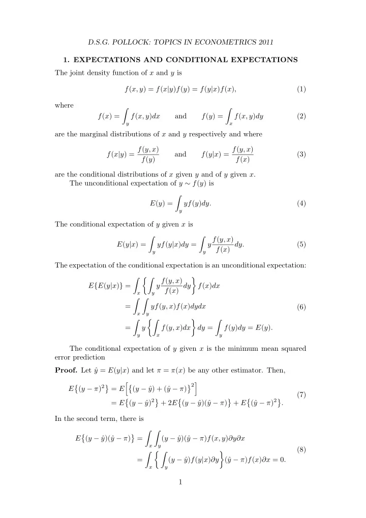
D.S.G. POLLOCK: TOPICS IN ECONOMETRICS 2011 1. EXPECTATIONS AND CONDITIONAL EXPECTATIONS The joint density function of x and y is f ( x, y ) = f ( x | y ) f ( y ) = f ( y | x ) f ( x ) , (1) where � � f ( x ) = f ( x, y ) dx and f ( y ) = f ( x, y ) dy (2) y x are the marginal distributions of x and y respectively and where f ( x | y ) = f ( y, x ) f ( y | x ) = f ( y, x ) and (3) f ( y ) f ( x ) are the conditional distributions of x given y and of y given x . The unconditional expectation of y ∼ f ( y ) is � E ( y ) = yf ( y ) dy. (4) y The conditional expectation of y given x is y f ( y, x ) � � E ( y | x ) = yf ( y | x ) dy = f ( x ) dy. (5) y y The expectation of the conditional expectation is an unconditional expectation: �� y f ( y, x ) � � E { E ( y | x ) } = f ( x ) dy f ( x ) dx x y � � = yf ( y, x ) f ( x ) dydx (6) x y �� � � � = y f ( y, x ) dx dy = f ( y ) dy = E ( y ) . y x y The conditional expectation of y given x is the minimum mean squared error prediction Proof. Let ˆ y = E ( y | x ) and let π = π ( x ) be any other estimator. Then, �� � 2 � ( y − π ) 2 � � E = E ( y − ˆ y ) + (ˆ y − π ) (7) y ) 2 � y − π ) 2 � � � � � = E ( y − ˆ + 2 E ( y − ˆ y )(ˆ y − π ) + E (ˆ . In the second term, there is � � � � E ( y − ˆ y )(ˆ y − π ) = ( y − ˆ y )(ˆ y − π ) f ( x, y ) ∂y∂x x y (8) � � � � = ( y − ˆ y ) f ( y | x ) ∂y (ˆ y − π ) f ( x ) ∂x = 0 . x y 1

D.S.G. POLLOCK: TOPICS IN ECONOMETRICS 2011 Therefore, E { ( y − π ) 2 } = E { ( y − ˆ y ) 2 } + E { (ˆ y − π ) 2 } ≥ E { ( y − ˆ y ) 2 } , and the assertion is proved. The error in predicting y is uncorrelated with x . The proof of this depends on showing that E (ˆ yx ) = E ( yx ), where ˆ y = E ( y | x ): � E (ˆ yx ) = xE ( y | x ) f ( x ) dx x �� y f ( y, x ) � � = x f ( x ) dy f ( x ) dx (9) x y � � = xyf ( y, x ) dydx = E ( xy ) . x y The result can be expressed as E { ( y − ˆ y ) x } = 0. This result can be used in deriving expressions for the parameters α and β of a linear regression of the form E ( y | x ) = α + βx, (10) from which and unconditional expectation is derived in the form of E ( y ) = α + βE ( x ) . (11) The orthogonality of the prediction error implies that 0 = E { ( y − ˆ y ) x } = E { ( y − α − βx ) x } (12) = E ( xy ) − αE ( x ) − βE ( x 2 ) . In order to eliminate αE ( x ) from this expression, equation (11) is multiplied by E ( x ) and rearranged to give αE ( x ) = E ( x ) E ( y ) − β { E ( x ) } 2 . (13) This substituted into (12) to give E ( x 2 ) − { E ( x ) } 2 � � E ( xy ) − E ( x ) E ( y ) = β , (14) whence β = E ( xy ) − E ( x ) E ( y ) = C ( x, y ) V ( x ) . (15) E ( x 2 ) − { E ( x ) } 2 The expression α = E ( y ) − βE ( x ) (16) comes directly from (9). Observe that, by substituting (16) into (10), the following prediction-error equation for the conditional expectation is derived: E ( y | x ) = E ( y ) + β { x − E ( x ) } . (17) 2

D.S.G. POLLOCK: TOPICS IN ECONOMETRICS 2011 Thus, the conditional expectation of y given x is obtained by adjusting the unconditional expectation by some proportion of the error in predicting x by its expected value. 2. THE PARTITIONED REGRESSSION MODEL Consider taking a regression equation in the form of � � β 1 y = [ X 1 X 2 ] + ε = X 1 β 1 + X 2 β 2 + ε. (1) β 2 2 ] ′ = β are obtained by partitioning the matrix X Here [ X 1 , X 2 ] = X and [ β ′ 1 , β ′ and vector β of the equation y = Xβ + ε in a conformable manner. The normal equations X ′ Xβ = X ′ y can be partitioned likewise. Writing the equations without the surrounding matrix braces gives X ′ 1 X 1 β 1 + X ′ 1 X 2 β 2 = X ′ 1 y, (2) X ′ 2 X 1 β 1 + X ′ 2 X 2 β 2 = X ′ 2 y. (3) From (2), we get the equation X ′ 1 X 1 β 1 = X ′ 1 ( y − X 2 β 2 ) which gives an expres- sion for the leading subvector of ˆ β : ˆ 1 ( y − X 2 ˆ 1 X 1 ) − 1 X ′ β 1 = ( X ′ β 2 ) . (4) To obtain an expression for ˆ β 2 , we must eliminate β 1 from equation (3). For 1 X 1 ) − 1 to give this purpose, we multiply equation (2) by X ′ 2 X 1 ( X ′ 1 X 1 ) − 1 X ′ 1 X 1 ) − 1 X ′ X ′ 2 X 1 β 1 + X ′ 2 X 1 ( X ′ 1 X 2 β 2 = X ′ 2 X 1 ( X ′ 1 y. (5) When the latter is taken from equation (3), we get � � 1 X 1 ) − 1 X ′ 1 X 1 ) − 1 X ′ X ′ 2 X 2 − X ′ 2 X 1 ( X ′ 1 X 2 β 2 = X ′ 2 y − X ′ 2 X 1 ( X ′ 1 y. (6) On defining 1 X 1 ) − 1 X ′ P 1 = X 1 ( X ′ 1 , (7) can we rewrite (6) as � � X ′ β 2 = X ′ 2 ( I − P 1 ) X 2 2 ( I − P 1 ) y, (8) whence � − 1 � ˆ X ′ X ′ β 2 = 2 ( I − P 1 ) X 2 2 ( I − P 1 ) y. (9) Now let us investigate the effect that conditions of orthogonality amongst the regressors have upon the ordinary least-squares estimates of the regression parameters. Consider a partitioned regression model, which can be written as � � β 1 y = [ X 1 , X 2 ] + ε = X 1 β 1 + X 2 β 2 + ε. (10) β 2 3

D.S.G. POLLOCK: TOPICS IN ECONOMETRICS 2011 It can be assumed that the variables in this equation are in deviation form. Imagine that the columns of X 1 are orthogonal to the columns of X 2 such that X ′ 1 X 2 = 0. This is the same as assuming that the empirical correlation between variables in X 1 and variables in X 2 is zero. The effect upon the ordinary least-squares estimator can be seen by exam- ining the partitioned form of the formula ˆ β = ( X ′ X ) − 1 X ′ y . Here we have � � � � � � X ′ X ′ 1 X 1 X ′ 1 X 2 X ′ 1 X 1 0 1 X ′ X = [ X 1 X 2 ] = = , (11) X ′ X ′ 2 X 1 X ′ 2 X 2 0 X ′ 2 X 2 2 where the final equality follows from the condition of orthogonality. The inverse of the partitioned form of X ′ X in the case of X ′ 1 X 2 = 0 is � − 1 � � 1 X 1 ) − 1 � X ′ 1 X 1 0 ( X ′ 0 ( X ′ X ) − 1 = = . (12) 2 X 2 ) − 1 0 X ′ 2 X 2 0 ( X ′ We also have � X ′ � X ′ 1 y � � 1 X ′ y = y = . (13) X ′ X ′ 2 y 2 On combining these elements, we find that � ˆ � ( X ′ � � X ′ � ( X ′ � 1 X 1 ) − 1 1 X 1 ) − 1 X ′ 0 1 y 1 y β 1 � � = = . (14) ˆ 2 X 2 ) − 1 2 X 2 ) − 1 X ′ 0 ( X ′ X ′ 2 y ( X ′ 2 y β 2 In this special case, the coefficients of the regression of y on X = [ X 1 , X 2 ] can be obtained from the separate regressions of y on X 1 and y on X 2 . It should be understood that this result does not hold true in general. The general formulae for ˆ β 1 and ˆ β 2 are those which we have given already under (4) and (9): ˆ 1 ( y − X 2 ˆ 1 X 1 ) − 1 X ′ β 1 = ( X ′ β 2 ) , (15) � − 1 X ′ ˆ 1 X 1 ) − 1 X ′ � X ′ P 1 = X 1 ( X ′ β 2 = 2 ( I − P 1 ) X 2 2 ( I − P 1 ) y, 1 . It can be confirmed easily that these formulae do specialise to those under (14) in the case of X ′ 1 X 2 = 0. The purpose of including X 2 in the regression equation when, in fact, interest is confined to the parameters of β 1 is to avoid falsely attributing the explanatory power of the variables of X 2 to those of X 1 . Let us investigate the effects of erroneously excluding X 2 from the regres- sion. In that case, the estimate will be ˜ 1 X 1 ) − 1 X ′ β 1 = ( X ′ 1 y 1 X 1 ) − 1 X ′ = ( X ′ 1 ( X 1 β 1 + X 2 β 2 + ε ) (16) 1 X 1 ) − 1 X ′ 1 X 1 ) − 1 X ′ = β 1 + ( X ′ 1 X 2 β 2 + ( X ′ 1 ε. 4