CSC304 Lectures 17-18 Voting 3: Axiomatic, Statistical, and - PowerPoint PPT Presentation
CSC304 Lectures 17-18 Voting 3: Axiomatic, Statistical, and Utilitarian Approaches to Voting CSC304 - Nisarg Shah 1 Recap We introduced a plethora of voting rules Plurality Plurality with runoff Borda Kemeny Veto
CSC304 Lectures 17-18 Voting 3: Axiomatic, Statistical, and Utilitarian Approaches to Voting CSC304 - Nisarg Shah 1
Recap • We introduced a plethora of voting rules ➢ Plurality ➢ Plurality with runoff ➢ Borda ➢ Kemeny ➢ Veto ➢ Copeland ➢ 𝑙 -Approval ➢ Maximin ➢ STV • Which is the right way to aggregate preferences? ➢ GS Theorem: There is no good strategyproof voting rule. ➢ For now, let us forget about incentives. Let us focus on how to aggregate given truthful votes. CSC304 - Nisarg Shah 2
Recap • Set of voters 𝑂 = {1, … , 𝑜} 1 2 3 • Set of alternatives 𝐵 , 𝐵 = 𝑛 a c b • Voter 𝑗 has a preference b a a ranking ≻ 𝑗 over the c b c alternatives • Preference profile ≻ = collection of all voter rankings • Voting rule (social choice function) 𝑔 ➢ Takes as input a preference profile ≻ ➢ Returns an alternative 𝑏 ∈ 𝐵 CSC304 - Nisarg Shah 3
Axiomatic Approach • Goal: Define a set of reasonable desiderata, and find voting rules satisfying them ➢ Ultimate hope: a unique voting rule satisfies the axioms we are interested in! • Sadly, it’s often the opposite case. ➢ Many combinations of reasonable axioms cannot be satisfied by any voting rule. ➢ GS theorem: nondictatorship + ontoness + strategyproofness = ∅ ➢ Arrow’s theorem: we’ll see ➢ … CSC304 - Nisarg Shah 4
Axiomatic Approach • Unanimity: If all voters have the same top choice, that alternative is the winner. 𝑢𝑝𝑞 ≻ 𝑗 = 𝑏 ∀𝑗 ∈ 𝑂 ⇒ 𝑔 ≻ = 𝑏 ➢ I used 𝑢𝑝𝑞 ≻ 𝑗 = 𝑏 to denote 𝑏 ≻ 𝑗 𝑐 ∀𝑐 ≠ 𝑏 • Pareto optimality: If all voters prefer 𝑏 to 𝑐 , then 𝑐 is not the winner. 𝑏 ≻ 𝑗 𝑐 ∀𝑗 ∈ 𝑂 ⇒ 𝑔 ≻ ≠ 𝑐 • Q: What is the relation between these axioms? ➢ Pareto optimality ⇒ Unanimity CSC304 - Nisarg Shah 5
Axiomatic Approach • Anonymity: Permuting votes does not change the winner (i.e., voter identities don’t matter). ➢ E.g., these two profiles must have the same winner: {voter 1 : 𝑏 ≻ 𝑐 ≻ 𝑑 , voter 2 : 𝑐 ≻ 𝑑 ≻ 𝑏 } {voter 1 : 𝑐 ≻ 𝑑 ≻ 𝑏 , voter 2 : 𝑏 ≻ 𝑐 ≻ 𝑑 } • Neutrality: Permuting the alternative names permutes the winner accordingly. ➢ E.g., say 𝑏 wins on {voter 1 : 𝑏 ≻ 𝑐 ≻ 𝑑 , voter 2 : 𝑐 ≻ 𝑑 ≻ 𝑏 } ➢ We permute all names: 𝑏 → 𝑐 , 𝑐 → 𝑑 , and 𝑑 → 𝑏 ➢ New profile: {voter 1 : 𝑐 ≻ 𝑑 ≻ 𝑏 , voter 2 : 𝑑 ≻ 𝑏 ≻ 𝑐 } ➢ Then, the new winner must be 𝑐 . CSC304 - Nisarg Shah 6
Axiomatic Approach • Neutrality is tricky ➢ As we defined it, it is inconsistent with anonymity! o Imagine {voter 1 : 𝑏 ≻ 𝑐 , voter 2 : 𝑐 ≻ 𝑏 } o Without loss of generality, say 𝑏 wins o Imagine a different profile: {voter 1: 𝑐 ≻ 𝑏, voter 2: 𝑏 ≻ 𝑐 } • Neutrality: We just exchanged 𝑏 ↔ 𝑐 , so winner is 𝑐 . • Anonymity: We just exchanged the votes, so winner stays 𝑏 . ➢ Typically, we only require neutrality for… o Randomized rules: E.g., a rule could satisfy both by choosing 𝑏 and 𝑐 as the winner with probability ½ each, on both profiles o Deterministic rules allowed to return ties: E.g., a rule could return {𝑏, 𝑐} as tied winners on both profiles. CSC304 - Nisarg Shah 7
Axiomatic Approach • Majority consistency: If a majority of voters have the same top choice, that alternative wins. > 𝑜 𝑗: 𝑢𝑝𝑞 ≻ 𝑗 = 𝑏 2 ⇒ 𝑔 ≻ = 𝑏 ➢ Satisfied by plurality, but not by Borda count • Condorcet consistency: If 𝑏 defeats every other alternative in a pairwise election, 𝑏 wins. > 𝑜 𝑗: 𝑏 ≻ 𝑗 𝑐 2 , ∀𝑐 ≠ 𝑏 ⇒ 𝑔 ≻ = 𝑏 ➢ Condorcet consistency ⇒ Majority consistency ➢ Violated by both plurality and Borda count CSC304 - Nisarg Shah 8
Axiomatic Approach • Is even the weaker axiom majority consistency a reasonable one to expect? 1 2 3 4 5 a a a b b b b b a a CSC304 - Nisarg Shah 9
Axiomatic Approach • Consistency: If 𝑏 is the winner on two profiles, it must be the winner on their union. 𝑔 ≻ 1 = 𝑏 ∧ 𝑔 ≻ 2 = 𝑏 ⇒ 𝑔 ≻ 1 +≻ 2 = 𝑏 ➢ Example: ≻ 1 = 𝑏 ≻ 𝑐 ≻ 𝑑 , ≻ 2 = 𝑏 ≻ 𝑑 ≻ 𝑐, 𝑐 ≻ 𝑑 ≻ 𝑏 ➢ Then, ≻ 1 +≻ 2 = 𝑏 ≻ 𝑐 ≻ 𝑑, 𝑏 ≻ 𝑑 ≻ 𝑐, 𝑐 ≻ 𝑑 ≻ 𝑏 • Is this reasonable? ➢ Young [1975] showed that subject to mild requirements, a voting rule is consistent if and only if it is a positional scoring rule! ➢ Thus, plurality with runoff, STV, Kemeny, Copeland, Maximin, etc are not consistent. CSC304 - Nisarg Shah 10
Axiomatic Approach • Weak monotonicity: If 𝑏 is the winner, and 𝑏 is “pushed up” in some votes, 𝑏 remains the winner. ➢ 𝑔 ≻ = 𝑏 ⇒ 𝑔 ≻ ′ = 𝑏 if ′ 𝑑, ∀𝑗 ∈ 𝑂, 𝑐, 𝑑 ∈ 𝐵\{𝑏} 1. 𝑐 ≻ 𝑗 𝑑 ⇔ 𝑐 ≻ 𝑗 “Order among other alternatives preserved in all votes” ′ 𝑐, ∀𝑗 ∈ 𝑂, 𝑐 ∈ 𝐵\{𝑏} 2. 𝑏 ≻ 𝑗 𝑐 ⇒ 𝑏 ≻ 𝑗 ( 𝑏 only improves) “In every vote, 𝑏 still defeats all the alternatives it defeated” • Contrast: strong monotonicity requires 𝑔 ≻ ′ = 𝑏 even if ≻ ′ only satisfies the 2 nd condition ➢ It is thus too strong. Equivalent to strategyproofness! ➢ Only satisfied by dictatorial/non-onto rules [GS theorem] CSC304 - Nisarg Shah 11
Axiomatic Approach • Weak monotonicity: If 𝑏 is the winner, and 𝑏 is “pushed up” in some votes, 𝑏 remains the winner. ➢ 𝑔 ≻ = 𝑏 ⇒ 𝑔 ≻ ′ = 𝑏 , where ′ 𝑑, ∀𝑗 ∈ 𝑂, 𝑐, 𝑑 ∈ 𝐵\{𝑏} (Order of others preserved) o 𝑐 ≻ 𝑗 𝑑 ⇔ 𝑐 ≻ 𝑗 ′ 𝑐, ∀𝑗 ∈ 𝑂, 𝑐 ∈ 𝐵\{𝑏} o 𝑏 ≻ 𝑗 𝑐 ⇒ 𝑏 ≻ 𝑗 ( 𝑏 only improves) • Weak monotonicity is satisfied by most voting rules ➢ Only exceptions (among rules we saw): STV and plurality with runoff ➢ But this helps STV be hard to manipulate o [Conitzer & Sandholm 2006]: “Every weakly monotonic voting rule is easy to manipulate on average.” CSC304 - Nisarg Shah 12
Axiomatic Approach • STV violates weak monotonicity 7 voters 5 voters 2 voters 6 voters 7 voters 5 voters 2 voters 6 voters a b b c a b a c b c c a b c b a c a a b c a c b • First 𝑑 , then 𝑐 eliminated • First 𝑐 , then 𝑏 eliminated • Winner: 𝑏 • Winner: 𝑑 CSC304 - Nisarg Shah 13
NOT IN Axiomatic Approach SYLLABUS • For social welfare functions that output a ranking: • Independence of Irrelevant Alternatives (IIA): ➢ If the preferences of all voters between 𝑏 and 𝑐 are unchanged, then the social preference between 𝑏 and 𝑐 should not change. • Arrow’s Impossibility Theorem ➢ No voting rule satisfies IIA, Pareto optimality, and nondictatorship. ➢ Proof omitted. ➢ Foundations of the axiomatic approach to voting CSC304 - Nisarg Shah 14
NOT IN Statistical Approach SYLLABUS • Assume that there is a “true” ranking of alternatives ➢ Unknown to us apriori • Votes {≻ 𝑗 } are generated i.i.d. from a distribution parametrized by a ranking 𝜏 ∗ ➢ Pr[≻ |𝜏 ∗ ] denotes the probability of drawing a vote ≻ given that the ground truth is 𝜏 ∗ • Maximum likelihood estimate (MLE): 𝑜 ➢ Given ≻ , return argmax 𝜏 Pr ≻ 𝜏 = ς 𝑗=1 Pr ≻ 𝑗 𝜏 CSC304 - Nisarg Shah 15
NOT IN Statistical Approach SYLLABUS • Example: Mallows’ model ➢ Recall Kendall-tau distance 𝑒 between two rankings: #pairs of alternatives on which they disagree ➢ Malllows ’ model: Pr ≻ 𝜏 ∗ ∝ 𝜒 𝑒 ≻,𝜏 ∗ , where o 𝜒 ∈ (0,1] is the “noise parameter” o 𝜒 → 0 : Pr 𝜏 ∗ 𝜏 ∗ → 1 o 𝜒 = 1 : uniform distribution o Normalization constant 𝑎 𝜒 = σ ≻ 𝜒 𝑒 ≻,𝜏 ∗ does not depend on 𝜏 ∗ ➢ The greater the distance from the ground truth, the smaller the probability CSC304 - Nisarg Shah 16
NOT IN Statistical Approach SYLLABUS • Example: Mallows’ model ➢ What is the MLE ranking for Mallows’ model? 𝑜 𝜒 𝑒 ≻ 𝑗 ,𝜏 ∗ 𝑜 𝑜 𝑒 ≻ 𝑗 ,𝜏 ∗ 𝜒 σ 𝑗=1 Pr ≻ 𝑗 𝜏 ∗ = max max ෑ ෑ = max 𝑎 𝜒 𝑎 𝜒 𝜏 𝜏 𝜏 𝑗=1 𝑗=1 ➢ The MLE ranking 𝜏 ∗ minimizes σ 𝑗=1 𝑜 𝑒(≻ 𝑗 , 𝜏 ∗ ) ➢ This is precisely the Kemeny ranking! • Statistical approach yields a unique rule, but is specific to the assumed distribution of votes CSC304 - Nisarg Shah 17
Utilitarian Approach • Each voter 𝑗 still submits a ranking ≻ 𝑗 ➢ But the voter has “implicit” numerical utilities { 𝑤 𝑗 𝑏 ≥ } 0 Σ 𝑏 𝑤 𝑗 𝑏 = 1 𝑏 ≻ 𝑗 𝑐 ⇒ 𝑤 𝑗 𝑏 ≥ 𝑤 𝑗 𝑐 • Goal: ➢ Select 𝑏 ∗ with the maximum social welfare σ 𝑗 𝑤 𝑗 𝑏 ∗ o Cannot always find this given only rankings from voters ➢ Refined goal: Select 𝑏 ∗ that gives the best worst-case approximation of welfare CSC304 - Nisarg Shah 18
Distortion • The distortion of a voting rule 𝑔 is its approximation ratio of social welfare, on the worst preference profile. σ 𝑗 𝑤 𝑗 𝑐 max 𝑐 𝑒𝑗𝑡𝑢 𝑔 = sup σ 𝑗 𝑤 𝑗 𝑔(≻) 𝑤𝑏𝑚𝑗𝑒 {𝑤 𝑗 } ➢ where each 𝑤 𝑗 is valid if Σ 𝑏 𝑤 𝑗 𝑏 = 1 ➢ ≻ = ≻ 1 , … , ≻ 𝑜 where ≻ 𝑗 represents the ranking of alternatives according to 𝑤 𝑗 CSC304 - Nisarg Shah 19
Recommend
More recommend
Explore More Topics
Stay informed with curated content and fresh updates.
