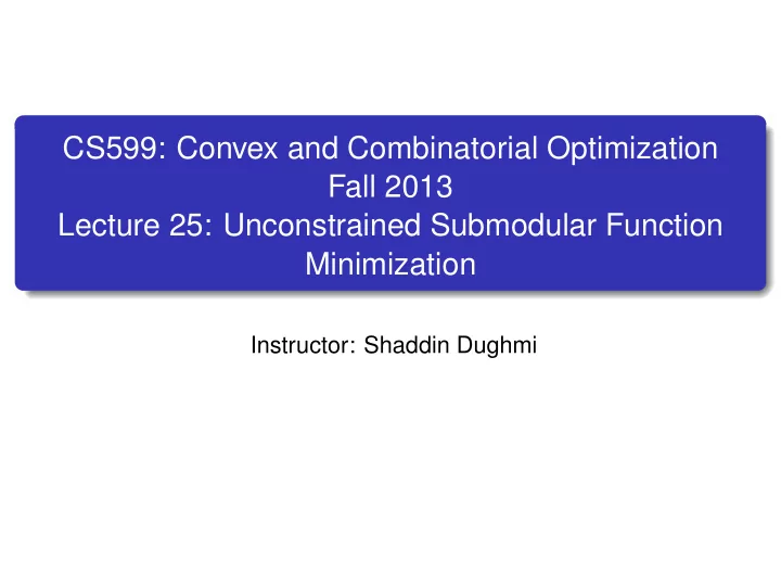
CS599: Convex and Combinatorial Optimization Fall 2013 Lecture 25: - PowerPoint PPT Presentation
CS599: Convex and Combinatorial Optimization Fall 2013 Lecture 25: Unconstrained Submodular Function Minimization Instructor: Shaddin Dughmi Announcements Outline Introduction 1 The Convex Closure and the Lovasz Extension 2 Wrapping up 3
CS599: Convex and Combinatorial Optimization Fall 2013 Lecture 25: Unconstrained Submodular Function Minimization Instructor: Shaddin Dughmi
Announcements
Outline Introduction 1 The Convex Closure and the Lovasz Extension 2 Wrapping up 3
Recall: Optimizing Submodular Functions As our examples suggest, optimization problems involving submodular functions are very common These can be classified on two axes: constrained/unconstrained and maximization/minimization Maximization Minimization Unconstrained NP-hard Polynomial time 1 2 approximation via convex opt Constrained Usually NP-hard Usually NP-hard to apx. 1 − 1 /e (mono, matroid) Few easy special cases O (1) (“nice” constriants) Introduction 1/17
Recall: Optimizing Submodular Functions As our examples suggest, optimization problems involving submodular functions are very common These can be classified on two axes: constrained/unconstrained and maximization/minimization Maximization Minimization Unconstrained NP-hard Polynomial time 1 2 approximation via convex opt Constrained Usually NP-hard Usually NP-hard to apx. 1 − 1 /e (mono, matroid) Few easy special cases O (1) (“nice” constriants) Introduction 1/17
Problem Definition Given a submodular function f : 2 X → R on a finite ground set X , minimize f ( S ) S ⊆ X subject to We denote n = | X | We assume f ( S ) is a rational number with at most b bits Introduction 2/17
Problem Definition Given a submodular function f : 2 X → R on a finite ground set X , minimize f ( S ) S ⊆ X subject to We denote n = | X | We assume f ( S ) is a rational number with at most b bits Representation In order to generalize all our examples, algorithmic results are often posed in the value oracle model. Namely, we only assume we have access to a subroutine evaluating f ( S ) in constant time. Introduction 2/17
Problem Definition Given a submodular function f : 2 X → R on a finite ground set X , minimize f ( S ) S ⊆ X subject to We denote n = | X | We assume f ( S ) is a rational number with at most b bits Representation In order to generalize all our examples, algorithmic results are often posed in the value oracle model. Namely, we only assume we have access to a subroutine evaluating f ( S ) in constant time. Goal An algorithm which runs in time polynomial in n and b . Introduction 2/17
Problem Definition Given a submodular function f : 2 X → R on a finite ground set X , minimize f ( S ) S ⊆ X subject to We denote n = | X | We assume f ( S ) is a rational number with at most b bits Representation In order to generalize all our examples, algorithmic results are often posed in the value oracle model. Namely, we only assume we have access to a subroutine evaluating f ( S ) in constant time. Goal An algorithm which runs in time polynomial in n and b . Note: weakly polynomial. There are strongly polytime algorithms. Introduction 2/17
Examples Minimum Cut Given a graph G = ( V, E ) , find a set S ⊆ V minimizing the number of edges crossing the cut ( S, V \ S ) . G may be directed or undirected. Extends to hypergraphs. Introduction 3/17
Examples Minimum Cut Given a graph G = ( V, E ) , find a set S ⊆ V minimizing the number of edges crossing the cut ( S, V \ S ) . G may be directed or undirected. Extends to hypergraphs. Densest Subgraph Given an undirected graph G = ( V, E ) , find a set S ⊆ V maximizing the average internal degree. Reduces to supermodular maximization via binary search for the right density. Introduction 3/17
Outline Introduction 1 The Convex Closure and the Lovasz Extension 2 Wrapping up 3
Continuous Extensions of a Set Function Recall A set function f on X = { 1 , . . . , n } with can be thought of as a map from the vertices { 0 , 1 } n of the n -dimensional hypercube to the real numbers. The Convex Closure and the Lovasz Extension 4/17
Continuous Extensions of a Set Function Recall A set function f on X = { 1 , . . . , n } with can be thought of as a map from the vertices { 0 , 1 } n of the n -dimensional hypercube to the real numbers. We will consider extensions of a set function to the entire hypercube. Extension of a Set Function Given a set function f : { 0 , 1 } n → R , an extension of f to the hypercube [0 , 1] n is a function g : [0 , 1] n → R satisfying g ( x ) = f ( x ) for every x ∈ { 0 , 1 } n . The Convex Closure and the Lovasz Extension 4/17
Continuous Extensions of a Set Function Recall A set function f on X = { 1 , . . . , n } with can be thought of as a map from the vertices { 0 , 1 } n of the n -dimensional hypercube to the real numbers. We will consider extensions of a set function to the entire hypercube. Extension of a Set Function Given a set function f : { 0 , 1 } n → R , an extension of f to the hypercube [0 , 1] n is a function g : [0 , 1] n → R satisfying g ( x ) = f ( x ) for every x ∈ { 0 , 1 } n . Long story short. . . We will exhibit an extension which is convex when f is submodular, and can be minimized efficiently. We will then show that minimizing it yields a solution to the submodular minimization problem. The Convex Closure and the Lovasz Extension 4/17
The Convex Closure Convex Closure Given a set function f : { 0 , 1 } n → R , the convex closure f − : [0 , 1] n → R of f is the point-wise greatest convex function under-estimating f on { 0 , 1 } n . The Convex Closure and the Lovasz Extension 5/17
The Convex Closure Convex Closure Given a set function f : { 0 , 1 } n → R , the convex closure f − : [0 , 1] n → R of f is the point-wise greatest convex function under-estimating f on { 0 , 1 } n . Geometric Intuition What you would get by placing a blanket under the plot of f and pulling up. f ( ∅ ) = 0 f ( { 1 } ) = f ( { 2 } ) = 1 f ( { 1 , 2 } ) = 1 f − ( x 1 , x 2 ) = max( x 1 , x 2 ) The Convex Closure and the Lovasz Extension 5/17
The Convex Closure Convex Closure Given a set function f : { 0 , 1 } n → R , the convex closure f − : [0 , 1] n → R of f is the point-wise greatest convex function under-estimating f on { 0 , 1 } n . Claim The convex closure exists for any set function. Proof If g 1 , g 2 : [0 , 1] n → R are convex under-estimators of f , then so is max { g 1 , g 2 } Holds for infinite set of convex under-estimators Therefore f − = max { g : g is a convex underestimator of f } is the point-wise greatest convex underestimator of f . The Convex Closure and the Lovasz Extension 5/17
Claim The value of the convex closure at x ∈ [0 , 1] n is the solution of the following optimization problem: minimize � y ∈{ 0 , 1 } n λ y f ( y ) y ∈{ 0 , 1 } n λ y y = x subject to � � y ∈{ 0 , 1 } n λ y = 1 for y ∈ { 0 , 1 } n . λ y ≥ 0 , Interpretation The minimum expected value of f over all distributions on { 0 , 1 } n with expectation x . Equivalently: the minimum expected value of f for a random set S ⊆ X including each i ∈ X with probability x i . The upper bound on f − ( x ) implied by applying Jensen’s inequality to every convex combination { 0 , 1 } n . The Convex Closure and the Lovasz Extension 6/17
Claim The value of the convex closure at x ∈ [0 , 1] n is the solution of the following optimization problem: minimize � y ∈{ 0 , 1 } n λ y f ( y ) y ∈{ 0 , 1 } n λ y y = x subject to � � y ∈{ 0 , 1 } n λ y = 1 for y ∈ { 0 , 1 } n . λ y ≥ 0 , Implication f − is a convex extension of f . f − ( x ) has no “integrality gap” For every x ∈ [0 , 1] n , there is a random integer vector y ∈ { 0 , 1 } n such that E y f ( y ) = f − ( x ) . Therefore, there is an integer vector y such that f ( y ) ≤ f − ( x ) . The Convex Closure and the Lovasz Extension 6/17
Claim The value of the convex closure at x ∈ [0 , 1] n is the solution of the following optimization problem: minimize � y ∈{ 0 , 1 } n λ y f ( y ) y ∈{ 0 , 1 } n λ y y = x subject to � � y ∈{ 0 , 1 } n λ y = 1 for y ∈ { 0 , 1 } n . λ y ≥ 0 , f ( ∅ ) = 0 f ( { 1 } ) = f ( { 2 } ) = 1 f ( { 1 , 2 } ) = 1 When x 1 ≤ x 2 f − ( x 1 , x 2 ) = x 1 f ( { 1 , 2 } ) + ( x 2 − x 1 ) f ( { 2 } ) + (1 − x 2 ) f ( ∅ ) The Convex Closure and the Lovasz Extension 6/17
Claim The value of the convex closure at x ∈ [0 , 1] n is the solution of the following optimization problem: minimize � y ∈{ 0 , 1 } n λ y f ( y ) y ∈{ 0 , 1 } n λ y y = x subject to � � y ∈{ 0 , 1 } n λ y = 1 for y ∈ { 0 , 1 } n . λ y ≥ 0 , Proof OPT ( x ) is at least f − ( x ) for every x : By Jensen’s inequality The Convex Closure and the Lovasz Extension 6/17
Claim The value of the convex closure at x ∈ [0 , 1] n is the solution of the following optimization problem: minimize � y ∈{ 0 , 1 } n λ y f ( y ) y ∈{ 0 , 1 } n λ y y = x subject to � � y ∈{ 0 , 1 } n λ y = 1 for y ∈ { 0 , 1 } n . λ y ≥ 0 , Proof OPT ( x ) is at least f − ( x ) for every x : By Jensen’s inequality To show that OPT ( x ) is equal to f − ( x ) , suffices to show that is a convex under-estimate of f The Convex Closure and the Lovasz Extension 6/17
Recommend
More recommend
Explore More Topics
Stay informed with curated content and fresh updates.
