
CS440/ECE448 Lecture 29: Review II Final Exam Mon, May 6, - PowerPoint PPT Presentation
CS440/ECE448 Lecture 29: Review II Final Exam Mon, May 6, 9:3010:45 Covers all lectures after the first exam. Same format as the first exam. Location (if youre in Prof. Hockenmaiers sections) Materials Science and Engineering
CS440/ECE448 Lecture 29: Review II
Final Exam Mon, May 6, 9:30–10:45 Covers all lectures after the first exam. Same format as the first exam. Location (if you’re in Prof. Hockenmaier’s sections) Materials Science and Engineering Building, Room 100 (http://ada.fs.illinois.edu/0034.html) Conflict exam: Wed, May 8, 9:30–10:45 Location: Siebel 3403. If you need to take your exam at DRES, make sure to notify DRES in advance
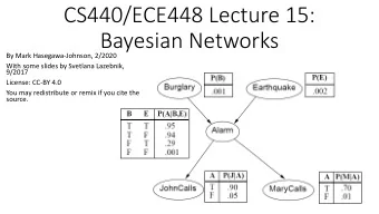
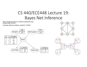
CS 440/ECE448 Lecture 19: Bayes Net Inference Mark Hasegawa-Johnson, 3/2019 modified by Julia Hockenmaier 3/2019 Including slides by Svetlana Lazebnik, 11/2016
Parameter learning Inference problem : given values of evidence variables • E = e , answer questions about query variables X using the posterior P( X | E = e ) Learning problem: estimate the parameters of the • probabilistic model P( X | E ) given a training sample {( x 1 , e 1 ), …, ( x n , e n )} Learning from complete observations: relative • frequency estimates Learning from data with missing observations: • EM algorithm
Missing data: the EM algorithm • The EM algorithm starts (“Expectation Maximization”) starts with an initial guess for each parameter value. • We try to improve the initial guess, using the algorithm on the next two slides: • E-step Training set • M-step C S R W 0.5? Sample 1 ? F T T 2 ? T F T 3 ? F F F 0.5? 0.5? 0.5? 0.5? 4 ? T T T 5 ? T F T 6 ? F T F 0.5? … … … …. … 0.5? 0.5? 0.5?
Missing data: the EM algorithm • E-Step (Expectation): Given the model parameters, replace each of the missing numbers with a probability (a number between 0 and 1) using !(" = 1, %, ', () ! " = 1 %, ', ( = ! " = 1, %, ', ( + !(" = 0, %, ', () Training set C S R W 0.5? Sample 1 0.5? F T T 2 0.5? T F T 3 0.5? F F F 0.5? 0.5? 0.5? 0.5? 4 0.5? T T T 5 0.5? T F T 6 0.5? F T F 0.5? … … … …. … 0.5? 0.5? 0.5?
Missing data: the EM algorithm • M-Step (Maximization): Given the missing data estimates, replace each of the missing model parameters using ! Variable = T Parents = value = 1[# times Variable = 5, Parents = value] 1[#times Parents = value] Training set C S R W 0.5 Sample 1 0.5? F T T 2 0.5? T F T 3 0.5? F F F 0.5 0.5 0.5 0.5 4 0.5? T T T 5 0.5? T F T 6 0.5? F T F 1.0 … … … …. … 1.0 0.5 0.0
CS440/ECE448 Lecture 20: Hidden Markov Models Slides by Svetlana Lazebnik, 11/2016 Modified by Mark Hasegawa-Johnson, 3/2019
Hidden Markov Models • At each time slice t , the state of the world is described by an unobservable (hidden) variable X t and an observable evidence variable E t • Transition model: The current state is conditionally independent of all the other states given the state in the previous time step Markov assumption : P(X t | X 0 , …, X t -1 ) := P(X t | X t -1 ) • Observation model: The evidence at time t depends only on the state at time t Markov assumption: P(E t | X 0: t , E 1: t -1 ) = P(E t | X t ) … X 2 X t -1 X t X 0 X 1 E 2 E t -1 E t E 1
Example Transition model state evidence Observation model
An alternative visualization U=T: 0.9 U=F: 0.1 0.3 0.7 R=T R=F 0.7 0.3 U=T: 0.2 U=F: 0.8 R t = T R t = F U t = T U t = F Observation Transition R t-1 = T 0.7 0.3 (emission) R t = T 0.9 0.1 probabilities probabilities R t-1 = F 0.3 0.7 R t = F 0.2 0.8
HMM Learning and Inference • Inference tasks • Filtering: what is the distribution over the current state X t given all the evidence so far, e 1:t • Smoothing: what is the distribution of some state X k given the entire observation sequence e 1:t ? • Evaluation: compute the probability of a given observation sequence e 1:t • Decoding: what is the most likely state sequence X 0:t given the observation sequence e 1:t ? • Learning • Given a training sample of sequences, learn the model parameters (transition and emission probabilities) • EM algorithm
CS440/ECE448 Lecture 21: Markov Decision Processes Slides by Svetlana Lazebnik, 11/2016 Modified by Mark Hasegawa-Johnson, 3/2019
Markov Decision Processes (MDPs) • Components that define the MDP. Depending on the problem statement, you either know these, or you learn them from data: • States s, beginning with initial state s 0 • Actions a • Each state s has actions A(s) available from it • Transition model P(s’ | s, a) • Markov assumption : the probability of going to s’ from s depends only on s and a and not on any other past actions or states • Reward function R(s) • Policy – the “solution” to the MDP: • p (s) ∈ A(s) : the action that an agent takes in any given state
Maximizing expected utility • The optimal policy p (s) should maximize the expected utility over all possible state sequences produced by following that policy: ! 1 23453673|2 9 = ; 2 9 < 23453673 "#$#% "%&'%()%" "#$*#+(, -*./ " 0 • How to define the utility of a state sequence ? • Sum of rewards of individual states • Problem: infinite state sequences • Solution: discount individual state rewards by a factor g between 0 and 1: = + g + g + 2 U ([ s , s , s , ! ]) R ( s ) R ( s ) R ( s ) ! 0 1 2 0 1 2 ¥ R å = g £ < g < t R ( s ) max ( 0 1 ) t - g 1 = t 0
Utilities of st states • Expected utility obtained by policy p starting in state s: ! " # = % 4 #5675895|#, < = = # ! #5675895 &'(') &)*+),-)& &'(.'/,0 1.23 & • The “true” utility of a state , denoted U(s), is the best possible expected sum of discounted rewards • if the agent executes the best possible policy starting in state s • Reminiscent of minimax values of states…
Finding the utilities of st states • If state s’ has utility U(s’), then Max node what is the expected utility of taking action a in state s ? å P ( s ' | s , a ) U ( s ' ) s ' Chance node • How do we choose the optimal P(s’ | s, a) action? å p = * ( s ) arg max P ( s ' | s , a ) U ( s ' ) Î a A ( s ) U(s’) s ' • What is the recursive expression for U(s) in terms of the utilities of its successor states? å = + g U ( s ) R ( s ) max P ( s ' | s , a ) U ( s ' ) a s '
The Bellman equation • Recursive relationship between the utilities of successive states: å = + g U ( s ) R ( s ) max P ( s ' | s , a ) U ( s ' ) Î a A ( s ) s ' • For N states, we get N equations in N unknowns • Solving them solves the MDP • Nonlinear equations -> no closed-form solution, need to use an iterative solution method (is there a globally optimum solution?) • We could try to solve them through expectiminimax search, but that would run into trouble with infinite sequences • Instead, we solve them algebraically • Two methods: value iteration and policy iteration
Method 1: Value iteration • Start out with every U ( s ) = 0 • Iterate until convergence • During the i th iteration, update the utility of each state according to this rule: å ¬ + g U ( s ) R ( s ) max P ( s ' | s , a ) U ( s ' ) + i 1 i Î a A ( s ) s ' • In the limit of infinitely many iterations, this is guaranteed to find the correct utility values • Error decreases exponentially, so in practice, don’t need an infinite number of iterations…
Method 2: Policy iteration • Start with some initial policy p 0 and alternate between the following steps: • Policy evaluation: calculate U p i ( s ) for every state s • Policy improvement: calculate a new policy p i +1 based on the updated utilities • Notice it’s kind of like hill-climbing in the N-queens problem. • Policy evaluation : Find ways in which the current policy is suboptimal • Policy improvement : Fix those problems • Unlike Value Iteration, this is guaranteed to converge in a finite number of steps , as long as the state space and action set are both finite .
Method 2, Step 1: Po Policy evaluation • Given a fixed policy p , calculate U p ( s ) for every state s å p p = + g p U ( s ) R ( s ) P ( s ' | s , ( s )) U ( s ' ) s ' • p (s) is fixed, therefore !(# $ |#, ' # ) is an #’×# matrix, therefore we can solve a linear equation to get U p ( s )! • Why is this “Policy Evaluation” formula so much easier to solve than the original Bellman equation? å = + g U ( s ) R ( s ) max P ( s ' | s , a ) U ( s ' ) Î a A ( s ) s '
CS 440/ECE448 Lecture 22: Reinforcement Learning Slides by Svetlana Lazebnik, 11/2016 Modified by Mark Hasegawa-Johnson, 4/2019 By Nicolas P. Rougier - Own work, CC BY-SA 3.0, https://commons.wikimedia.org/w/index.php?curid=29327040
Reinforcement learning strategies • Model-based • Learn the model of the MDP ( transition probabilities and rewards ) and try to solve the MDP concurrently • Model-free • Learn how to act without explicitly learning the transition probabilities P(s’ | s, a) • Q-learning: learn an action-utility function Q(s,a) that tells us the value of doing action a in state s
Recommend


More recommend
Explore More Topics
Stay informed with curated content and fresh updates.