CS440/ECE448 Lecture 10: Two-Player Games Slides by Mark - PowerPoint PPT Presentation
CS440/ECE448 Lecture 10: Two-Player Games Slides by Mark Hasegawa-Johnson & Svetlana Lazebnik, 2/2020 Distributed under CC-BY 4.0 (https://creativecommons.org/licenses/by/4.0/). You are free to share and/or adapt if you give attribution.
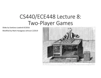
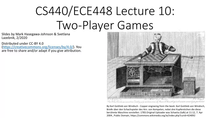
CS440/ECE448 Lecture 10: Two-Player Games Slides by Mark Hasegawa-Johnson & Svetlana Lazebnik, 2/2020 Distributed under CC-BY 4.0 (https://creativecommons.org/licenses/by/4.0/). You are free to share and/or adapt if you give attribution. By Karl Gottlieb von Windisch - Copper engraving from the book: Karl Gottlieb von Windisch, Briefe über den Schachspieler des Hrn. von Kempelen, nebst drei Kupferstichen die diese berühmte Maschine vorstellen. 1783.Original Uploader was Schaelss (talk) at 11:12, 7. Apr 2004., Public Domain, https://commons.wikimedia.org/w/index.php?curid=424092
Why study games? • Games are a traditional hallmark of intelligence • Games are easy to formalize • Games can be a good model of real-world competitive or cooperative activities • Military confrontations, negotiation, auctions, etc.
Game AI: Origins • Minimax algorithm: Ernst Zermelo, 1912 • Chess playing with evaluation function, quiescence search, selective search: Claude Shannon, 1949 (paper) • Alpha-beta search: John McCarthy, 1956 • Checkers program that learns its own evaluation function by playing against itself: Arthur Samuel, 1956
Types of game environments Deterministic Stochastic Perfect Backgammon, Chess, checkers, information monopoly go (fully observable) Battleship Imperfect Scrabble, information poker, (partially bridge observable)
Zero-sum Games
Alternating two-player zero-sum games • Players take turns • Each game outcome or terminal state has a utility for each player (e.g., 1 for win, 0 for loss) • The sum of both players’ utilities is a constant
Games vs. single-agent search • We don’t know how the opponent will act • The solution is not a fixed sequence of actions from start state to goal state, but a strategy or policy (a mapping from state to best move in that state)
Game tree • A game of tic-tac-toe between two players, “max” and “min”
http://xkcd.com/832/
A more abstract game tree Terminal utilities (for MAX) A two-ply game
Minimax Search
The rules of every game • Every possible outcome has a value (or “utility”) for me. • Zero-sum game: if the value to me is +V, then the value to my opponent is –V. • Phrased another way: • My rational action, on each move, is to choose a move that will maximize the value of the outcome • My opponent’s rational action is to choose a move that will minimize the value of the outcome • Call me “Max” • Call my opponent “Min”
Game tree search 3 3 2 2 • Minimax value of a node : the utility (for MAX) of being in the corresponding state, assuming perfect play on both sides • Minimax strategy: Choose the move that gives the best worst-case payoff
Computing the minimax value of a node 3 3 2 2 • Minimax ( node ) = § Utility( node ) if node is terminal § max action Minimax (Succ( node, action )) if player = MAX § min action Minimax (Succ( node, action )) if player = MIN
Optimality of minimax • The minimax strategy is optimal against an optimal opponent • What if your opponent is suboptimal? • Your utility will ALWAYS BE HIGHER than if you were playing an optimal opponent! • A different strategy may work better for a sub-optimal opponent, but it will necessarily be worse against an optimal opponent 11 Example from D. Klein and P. Abbeel
Multi-player games; Non-zero-sum games • More than two players. For example: • Dog ( 🐷 ) tries to maximize the number of doggie treats • Cat ( 🐲 ) tries to maximize the number of cat treats • Mouse ( 🐮 ) tries to maximize the number of mouse treats • Non-zero-sum. We can’t just assume that Min’s score is the opposite of Max’s. Instead, utilities are now tuples. For example: • ( 🐷 5, 🐲 8, 🐮 2) = 5 doggie treats, 8 kitty treats, 2 mouse treats • Each player maximizes their own utility at their node
Minimax in multi-player & non-zero-sum games ( 🐷 2, 🐲 5, 🐮 2) 🐷 ( 🐷 1, ( 🐷 2, 🐲 🐲 🐲 2, 🐲 5, 🐮 6) 🐮 2) ( 🐷 1, ( 🐷 2, ( 🐷 6, ( 🐷 5, 🐮 🐮 🐮 🐮 🐲 2, 🐲 5, 🐲 1, 🐲 4, 🐮 6) 🐮 2) 🐮 2) 🐮 5) ( 🐷 2, ( 🐷 1, ( 🐷 4, ( 🐷 5, ( 🐷 5, ( 🐷 6, ( 🐷 7, ( 🐷 7, 🐲 5, 🐲 2, 🐲 3, 🐲 1, 🐲 7, 🐲 4, 🐲 1, 🐲 4, 🐮 2) 🐮 6) 🐮 2) 🐮 1) 🐮 5) 🐮 2) 🐮 1) 🐮 1)
Alpha-Beta Pruning
Alpha-beta pruning • It is possible to compute the exact minimax decision without expanding every node in the game tree
Alpha-beta pruning • It is possible to compute the exact minimax decision without expanding every node in the game tree ³ 3 3
Alpha-beta pruning • It is possible to compute the exact minimax decision without expanding every node in the game tree ³ 3 3 £ 2
Alpha-beta pruning • It is possible to compute the exact minimax decision without expanding every node in the game tree ³ 3 3 £ 2 £ 14
Alpha-beta pruning • It is possible to compute the exact minimax decision without expanding every node in the game tree ³ 3 3 £ 2 £ 5
Alpha-beta pruning • It is possible to compute the exact minimax decision without expanding every node in the game tree 3 3 £ 2 2
Alpha-Beta Pruning Key point that I find most counter-intuitive: • MIN needs to calculate which move MAX will make. • MAX would never choose a suboptimal move. • So if MIN discovers that, at a particular node in the tree, she can make a move that’s REALLY REALLY GOOD for her… • She can assume that MAX will never let her reach that node. • … and she can prune it away from the search, and never consider it again.
Alpha-beta pruning • α is the value of the best choice for the MAX player found so far at any choice point above node n • More precisely: α is the highest number that MAX knows how to force MIN to accept • We want to compute the MIN-value at n • As we loop over n ’s children, the MIN-value decreases • If it drops below α , MAX will never choose n , so we can ignore n ’s remaining children
Alpha-beta pruning • β is the value of the best choice for the MIN player found so far β at any choice point above node n • More precisely: β is the lowest number that MIN know how to force MAX to accept • We want to compute the MAX-value at m • As we loop over m ’s children, the MAX-value increases m • If it rises above β , MIN will never choose m , so we can ignore m ’s remaining children
Alpha-beta pruning An unexpected result: • α is the highest number that MAX β knows how to force MIN to accept • β is the lowest number that MIN know how to force MAX to accept So 𝛽 ≤ 𝛾 m
Alpha-beta pruning Function action = Alpha-Beta-Search ( node ) v = Min-Value ( node , −∞, ∞) node return the action from node with value v α: best alternative available to the Max player action β: best alternative available to the Min player … Function v = Min-Value ( node , α , β ) Succ( node , action ) if Terminal( node ) return Utility( node ) v = +∞ for each action from node v = Min( v , Max-Value (Succ( node , action ), α , β )) if v ≤ α return v β = Min( β , v ) end for return v
Alpha-beta pruning Function action = Alpha-Beta-Search ( node ) v = Max-Value ( node , −∞, ∞) node return the action from node with value v α: best alternative available to the Max player action β: best alternative available to the Min player … Function v = Max-Value ( node , α , β ) Succ( node , action ) if Terminal( node ) return Utility( node ) v = −∞ for each action from node v = Max( v , Min-Value (Succ( node , action ), α , β )) if v ≥ β return v α = Max( α , v ) end for return v
Alpha-beta pruning • Pruning does not affect final result • Amount of pruning depends on move ordering • Should start with the “best” moves (highest-value for MAX or lowest-value for MIN) • For chess, can try captures first, then threats, then forward moves, then backward moves • Can also try to remember “killer moves” from other branches of the tree • With perfect ordering, the time to find the best move is reduced to O(b m/2 ) from O(b m ) • Depth of search is effectively doubled
Limited-Horizon Computation
Games vs. single-agent search • We don’t know how the opponent will act • The solution is not a fixed sequence of actions from start state to goal state, but a strategy or policy (a mapping from state to best move in that state)
Games vs. single-agent search • We don’t know how the opponent will act • The solution is not a fixed sequence of actions from start state to goal state, but a strategy or policy (a mapping from state to best move in that state) • Efficiency is critical to playing well • The time to make a move is limited • The branching factor, search depth, and number of terminal configurations are huge • In chess, branching factor ≈ 35 and depth ≈ 100, giving a search tree of 10 154 nodes • Number of atoms in the observable universe ≈ 10 80 • This rules out searching all the way to the end of the game
Recommend
More recommend
Explore More Topics
Stay informed with curated content and fresh updates.
