Crises and Prices: Information Aggregation, Multiplicity, and - - PowerPoint PPT Presentation

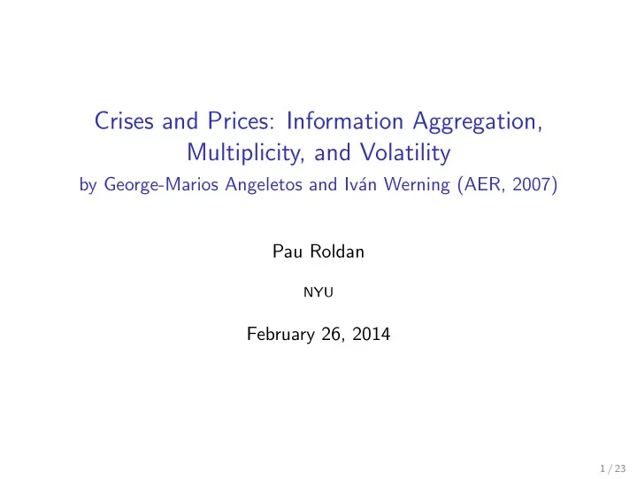
Crises and Prices: Information Aggregation, Multiplicity, and Volatility

by George-Marios Angeletos and Iv´ an Werning (AER, 2007) Pau Roldan

NYU

February 26, 2014

1 / 23

Motivation

Exogenous versus endogenous information

◮ Crises are times of high nonfundamental volatility in which

informative variables are being closely monitored.

◮ This model:

◮ Introduction of a financial market in a coordination game with

imperfect information.

◮ Information will be endogenous (through equilibrium

• utcomes).

◮ Asset price aggregates dispersed private information and will

act as a public noisy signal.

◮ Results:

◮ Uniqueness may no longer obtain as a perturbation from

perfect information

◮ Sunspots will deliver nonfundamental volatility in crises. ◮ Nonfundamental volatility may arise when agents use sunspots

to coordinate on different equilibria.

2 / 23

Motivation

Exogenous versus endogenous information (ctd.)

◮ Aim is to study role of endogenous information during crises:

◮ Investigate nonfundamental volatility arising from sunspots

(multiplicity of equilibria).

◮ Examine, when there is uniqueness, sensitivity of outcomes to

nonfundamental disturbances (noise in public signals).

◮ Main insight:

◮ Precision of endogenous public information increases with the

precision of exogenous private information.

◮ If private signals are more precise, asset demands are more

sensitive and equilibrium prices react more to fundamental than to non fundamental variables, conveying more precise information.

3 / 23

Motivation

Coordination: Uniqueness versus multiplicity

◮ More precise public information allows individuals to forecast

• ne another’s actions and allows easier coordination.

◮ This gives rise to multiplicity when information (private or

public) has little noise:

4 / 23

Outline

Motivation Model Exogenous Information Endogenous Information Extensions Extension 1: Price Multiplicity Extension 2: Observing One Another Conclusions

5 / 23

Outline

Motivation Model Exogenous Information Endogenous Information Extensions Extension 1: Price Multiplicity Extension 2: Observing One Another Conclusions

6 / 23

Baseline: Exogenous Information

Basic Setting

◮ Measure-one continuum of agents, i ∈ [0, 1]. ◮ Choice of action ai ∈ {0, 1} (attack status quo or not).

◮ Cost c ∈ (0, 1) of attacking.

◮ Let A :=

1

0 aidi be size of attack, θ an exogenous

fundamental.

◮ Status quo is abandoned (attack is successful) if A > θ. ◮ Individual payoff:

U(ai, A, θ) := ai(1[A>θ] − c)

◮ Coordination: U(1, A, θ) − U(0, A, θ) increases with A.

7 / 23

Baseline: Exogenous Information

Information structure

◮ State θ is not common knowledge (imperfect information). ◮ Common diffuse prior: Nature draws θ ∼ unif (−∞, +∞). ◮ Private signals: Mutually independent, uncorrelated with θ.

xi = θ + σxξi, ξi ∼ N(0, 1)

◮ Exogenous (for now) public signal:

z = θ + σzε, ε ∼ N(0, 1)

◮ Denote precisions by:

αx := σ−2

x

and αz := σ−2

z

8 / 23

Baseline: Exogenous Information

Symmetric Perfect Bayesian Equilibrium

◮ As in Morris and Shin, focus is on monotone PBE. ◮ For each z, agent i will attack iff xi ≤ x⋆(z). ◮ Aggregate size of attack is A(θ, z) = P[x ≤ x⋆(z)|θ]. ◮ Status quo is abandoned if θ ≤ θ⋆(z), where θ⋆(z) solves

A(θ, z) = θ, or x⋆(z) = θ⋆(z) + 1 √αx Φ−1[θ⋆(z)] (1)

◮ x⋆(z) solves indifference condition P[θ ≤ θ⋆(z)|x, z] = c, or

Φ √αx + αz

• θ⋆(z) − αxx⋆(z) + αzz

αx + αz

• = c

(2)

◮ Equilibrium is the joint solution to (1) and (2).

9 / 23

Baseline: Exogenous Information

Symmetric Perfect Bayesian Equilibrium (ctd.)

Proposition (Morris and Shin)

The equilibrium is unique iff private noise is small relative to public noise: σx σ2

z

≤ √ 2π

◮ Intuition:

◮ When private information is more diverse, it is more difficult

for individuals to predict the actions of others.

◮ When this effect is strong enough, multiplicity breaks down. 10 / 23

Outline

Motivation Model Exogenous Information Endogenous Information Extensions Extension 1: Price Multiplicity Extension 2: Observing One Another Conclusions

11 / 23

Endogenous Information

Motivation

◮ Until now, private and public noise were independent from

each other because information structure was exogenous.

◮ Any small noise away from perfect information (where

σx = σz = 0) ensured uniqueness (Morris and Shin).

◮ Thus, non fundamental volatility disappears when private

noise vanishes.

◮ Now, introduce a financial market where agents can trade

prior to the coordination game.

◮ Dividends will depend on aggregate attack and equilibrium

prices will convey information.

12 / 23

Endogenous Information

Setting

◮ Nature draws θ ∼ unif (−∞, +∞). ◮ Private signal for agent i:

xi = θ + σxξi, σx > 0, ξi ∼ N(0, 1)

◮ First stage:

◮ Trade over risky asset with dividend f (θ) of price p. ◮ Utility of agent i:

V(wi) = −e−γwi, γ > 0 wi = w0 − pki + fki where ki is investment in risky asset.

◮ Stochastic asset supply (prices are not fully revealing):

K s(ε) = σεε, σε > 0, ε ∼ N(0, 1)

◮ σε is exogenous noise in aggregation process. 13 / 23

Endogenous Information

Setting (ctd.)

◮ Second stage:

◮ After trade, agents observe stage-1 price p and choose whether

• r not to attack status quo.

◮ Utility for agent i:

U(ai, A, θ) = ai(1[A>θ] − c) where A := 1

0 aidi.

◮ Regime outcome, asset’s dividend and payoffs from both

stages realized at the end of stage 2.

◮ Equilibrium definition combines rational-expectations

equilibrium (first stage) and PBE (second stage).

14 / 23

Endogenous Information

Equilibrium definition

Definition

• 1. An equilibrium is a price function P(θ, ε), individual strategies

for investment and attacking, k(x, p) and a(x, p), and their corresponding aggregates, K(θ, p) and A(θ, p), such that: k(x, p) ∈ arg max

k∈R

E[V(w0 + (f (θ) − p)k)|x, p] K(θ, p) = E[k(x, p)|θ, p] K(θ, P(θ, ε)) = K s(ε) a(x, p) ∈ arg max

a∈{0,1} E[U(a, A(θ, p), θ)|x, p]

A(θ, p) = E[a(x, p)|θ, p]

• 2. The equilibrium regime outcome is R(θ, ε) := 1[A(θ,P(θ,ε))>θ].

15 / 23

Endogenous Information

Equilibrium analysis

◮ Use f (θ) = θ. ◮ Guess a linear price function that is not perfectly revealing.

◮ Price is a normally distributed public signal with precision αp. ◮ By Bayes’ rule:

θ|x, p ∼ N αxx + αpp αx + αp , 1 αx + αp

• ◮ Equilibrium asset demand (Grossman and Stiglitz (1980)):

k(x, p) = E[f (θ)|x, p] − p γV[f (θ)|x, p] = αx(x − p) γ

◮ Equilibrium price:

P(θ, ε) = θ − σpε

16 / 23

Endogenous Information

Equilibrium analysis (ctd.)

◮ Linear price guess is verified for:

σp = γσεσ2

x ◮ Thus, unlike before, public information improves with private

information (lower σx means lower σp).

◮ Before: ◮ Precision of public information was fixed, so that sufficiently

precise private information ensured uniqueness.

◮ Now: ◮ Better private information improves public information and

reduces strategic uncertainty to ensure multiplicity.

◮ There is multiplicity even for a small deviation of σx or σp

from zero (the perfect-information benchmark).

◮ Crises (periods of high nonfundamental volatility) can be

addressed even when σx → 0.

17 / 23

Endogenous Information

Equilibrium analysis (ctd.)

Proposition

There are multiple equilibria if either source of noise is small is small, so that σ2

εσ3 x < 1 γ2√ 2π.

Proposition

As either source of noise vanishes (σx → 0 or σε → 0),

• 1. There exists a passive equilibrium such that

R(θ, ε) → 0, ∀θ ∈ (θ, θ)

• 2. There exists an aggressive equilibrium such that

R(θ, ε) → 1, ∀θ ∈ (θ, θ)

◮ That is, unlike in the baseline Morris and Shin, regime

• utcome is fully sunspot-driven!

18 / 23

Outline

Motivation Model Exogenous Information Endogenous Information Extensions Extension 1: Price Multiplicity Extension 2: Observing One Another Conclusions

19 / 23

Price Multiplicity

◮ Before, financial market (first stage) endogenously provided

information to coordination game (second stage) through prices.

◮ Now, feedback is in the opposite direction as well. ◮ This will give multiplicity also in the equilibrium price. ◮ Setting:

◮ Same as before, except now dividend is endogenous, a function

• f the aggregate state:

f ≡ f (A) = −Φ−1(A)

◮ Linear monotone equilibrium features:

◮ σp = γσεσx, i.e. public info improves again with private info. ◮ Backward-bending asset demand K(θ, p), thus price

multiplicity in a non-empty parameter region of (θ, ε).

20 / 23

Outline

Motivation Model Exogenous Information Endogenous Information Extensions Extension 1: Price Multiplicity Extension 2: Observing One Another Conclusions

21 / 23

Observing One Another

◮ Now, remove financial market and focus on situations where

information originates within coordination game itself.

◮ Direct public signal on actions:

y = S(A, ε) where ε is independent of θ and ξ.

Definition

An equilibrium is an endogenous signal y = Y (θ, ε), an individual attack strategy a(x, y) and aggregate attack A(θ, y) such that a(x, y) = arg max

a∈[0,1] E[U(a, A(θ.y), θ)|x, y]

A(θ, y) = E[a(x, y)|θ, y] y = S(A(θ, y), ε)

◮ Once again, multiplicity iff either noise is small: σ2 εσx < 1 √ 2π.

22 / 23

Takeaways

◮ Exogenous information:

◮ Multiplicity disappears when agents observe fundamentals with

small private noise.

◮ No sunspot volatility for σx small enough. ◮ All non fundamental volatility vanishes and regime outcome is

independent of ε.

◮ Endogenous information:

◮ Multiplicity does not disappear for small noises (if public info

precision increases faster than square root of private info precision).

◮ Potential sunspot volatility is greatest when either noise

vanishes.

◮ Regime outcome and attack size are sunspot-driven as noise

vanishes.

23 / 23