Credits and the Instability of the Financial System: a Physicists - PowerPoint PPT Presentation

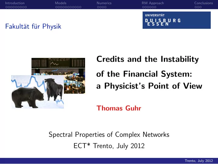
Introduction Models Numerics RM Approach Conclusions Fakult¨ at f¨ ur Physik Credits and the Instability of the Financial System: a Physicist’s Point of View Thomas Guhr Spectral Properties of Complex Networks ECT* Trento, July 2012 Trento, July 2012

Introduction Models Numerics RM Approach Conclusions Outline ◮ Introduction — econophysics, credit risk ◮ Structural model and loss distribution ◮ Numerical simulations and random matrix approach ◮ Conclusions — general, present credit crisis Trento, July 2012

Introduction Models Numerics RM Approach Conclusions Introduction — Econophysics Trento, July 2012

Introduction Models Numerics RM Approach Conclusions Some History: Connection Physics–Economics Trento, July 2012

Introduction Models Numerics RM Approach Conclusions Some History: Connection Physics–Economics Einstein 1905 Bachelier 1900 Trento, July 2012

Introduction Models Numerics RM Approach Conclusions Some History: Connection Physics–Economics Einstein 1905 Bachelier 1900 Trento, July 2012

Introduction Models Numerics RM Approach Conclusions Some History: Connection Physics–Economics Einstein 1905 Bachelier 1900 Mandelbrot 60’s Trento, July 2012

Introduction Models Numerics RM Approach Conclusions Growing Jobmarket for Physicists “Every tenth academic hired by Deutsche Bank is a natural scientist.” Trento, July 2012

Introduction Models Numerics RM Approach Conclusions A New Interdisciplinary Direction in Basic Research Theoretical physics: construction and analysis of mathematical models based on experiments or empirical information physics − → economics: much better economic data now, growing interest in complex systems Study economy as complex system in its own right economics − → physics: risk managment, expertise in model building based on empirical data Trento, July 2012

Introduction Models Numerics RM Approach Conclusions Economics — a Broad Range of Different Aspects Psychology Laws and Regulations ECONOMICS Ethics Politics Business Administration Quantitative Problems Trento, July 2012

Introduction Models Numerics RM Approach Conclusions Example: Return Distributions R ∆ t ( t ) = S ( t + ∆ t ) − S ( t ) S ( t ) non–Gaussian, heavy tails! (Mantegna, Stanley, ..., 90’s) Trento, July 2012

Introduction Models Numerics RM Approach Conclusions Introduction — Credit Risk Trento, July 2012

Introduction Models Numerics RM Approach Conclusions Credits and Stability of the Economy ◮ credit crisis shakes economy − → dramatic instability Trento, July 2012

Introduction Models Numerics RM Approach Conclusions Credits and Stability of the Economy ◮ credit crisis shakes economy − → dramatic instability ◮ claim: risk reduction by diversification Trento, July 2012

Introduction Models Numerics RM Approach Conclusions Credits and Stability of the Economy ◮ credit crisis shakes economy − → dramatic instability ◮ claim: risk reduction by diversification ◮ questioned with qualitative reasoning by several economists Trento, July 2012

Introduction Models Numerics RM Approach Conclusions Credits and Stability of the Economy ◮ credit crisis shakes economy − → dramatic instability ◮ claim: risk reduction by diversification ◮ questioned with qualitative reasoning by several economists ◮ I now present our quantitative study and answer Trento, July 2012

Introduction Models Numerics RM Approach Conclusions Defaults and Losses ◮ default occurs if obligor fails to repay → loss ◮ possible losses have to be priced into credit contract ◮ correlations are important to evaluate risk of credit portfolio ◮ statistical model to estimate loss distribution Trento, July 2012

Introduction Models Numerics RM Approach Conclusions Zero–Coupon Bond t = 0 Creditor Obligor Principal t = T Creditor Obligor Face value ◮ principal: borrowed amount ◮ face value F : borrowed amount + interest + risk compensation ◮ credit contract with simplest cash-flow ◮ credit portfolio comprises many such contracts Trento, July 2012

Introduction Models Numerics RM Approach Conclusions Modeling Credit Risk Trento, July 2012

Introduction Models Numerics RM Approach Conclusions Structural Models of Merton Type V k ( t ) V k (0) F T t ◮ microscopic approach for K companies ◮ economic state: risk elements V k ( t ) , k = 1 , . . . , K ◮ default occurs if V k ( T ) falls below face value F k ◮ then the (normalized) loss is L k = F k − V k ( T ) F k Trento, July 2012

Introduction Models Numerics RM Approach Conclusions Geometric Brownian Motion with Jumps K companies, risk elements V k ( t ) , k = 1 , . . . , K represent economic states, closely related to stock prices √ dV k ( t ) V k ( t ) = µ k dt + σ k ε k ( t ) dt + dJ k ( t ) we include jumps ! ◮ drift term (deterministic) µ k dt √ ◮ diffusion term (stochastic) σ k ε k ( t ) dt ◮ jump term (stochastic) dJ k ( t ) parameters can be tuned to describe the empirical distributions Trento, July 2012

Introduction Models Numerics RM Approach Conclusions Jump Process and Price or Return Distributions V k ( t ) with jumps without jumps V k (0) jump t jumps reproduce empirically found heavy tails Trento, July 2012

Introduction Models Numerics RM Approach Conclusions Financial Correlations 1.3 IBM asset values V k ( t ′ ) , k = 1 , . . . , K MSFT 1.2 measured at t ′ = 1 , . . . , T ′ 1.1 S(t) / S(Jan 2008) 1.0 0.9 returns R k ( t ′ ) = dV k ( t ′ ) 0.8 0.7 V k ( t ′ ) 0.6 Jan 2008 Feb 2008 Mar 2008 Apr 2008 May 2008 Jun 2008 Jul 2008 Aug 2008 Sep 2008 Oct 2008 Nov 2008 Dec 2008 R k ( t ′ ) − � R k ( t ′ ) � normalization M k ( t ′ ) = � � R 2 k ( t ′ ) � − � R k ( t ′ ) � 2 T ′ � u ( t ′ ) � = 1 � correlation C kl = � M k ( t ′ ) M l ( t ′ ) � , u ( t ′ ) T ′ t ′ =1 K × T ′ data matrix M such that C = 1 T ′ MM † Trento, July 2012

Introduction Models Numerics RM Approach Conclusions Inclusion of Correlations in Risk Elements ◮ ε i ( t ) , i = 1 , . . . , I set of random variables ◮ K × I structure matrix A ◮ correlated diffusion, uncorrelated drift, uncorrelated jumps I √ dV k ( t ) � V k ( t ) = µ k dt + σ k A ki ε i ( t ) dt + dJ k ( t ) i =1 for T → ∞ correlation matrix is C = AA † covariance matrix is Σ = σ C σ with σ = diag ( σ 1 , . . . , σ K ) Trento, July 2012

Introduction Models Numerics RM Approach Conclusions Loss Distribution Trento, July 2012

Introduction Models Numerics RM Approach Conclusions Individual Losses normalized loss at maturity V k ( t ) t = T V k (0) L k = F k − V k ( T ) Θ( F k − V k ( T )) F F k T t if default occurs Trento, July 2012

Introduction Models Numerics RM Approach Conclusions Portfolio Loss Distribution ◮ homogeneous portfolio K ◮ portfolio loss L = 1 � L k K k =1 ◮ stock prices at maturity V = ( V 1 ( T ) , . . . , V K ( T )) ◮ distribution p (mv) ( V , Σ) with Σ = σ C σ want to calculate � K � L − 1 � � d [ V ] p (mv) ( V , Σ) δ p ( L ) = L k K k =1 Trento, July 2012

Introduction Models Numerics RM Approach Conclusions Large Portfolios Real portfolios comprise several hundred or more individual contracts − → K is large. Central Limit Theorem: For very large K , portfolio loss distribution p ( L ) must become Gaussian. Question: how large is “very large” ? Trento, July 2012

Introduction Models Numerics RM Approach Conclusions Typical Portfolio Loss Distributions Frequency Unexpected loss Expected loss α -quantile Loss in % of exposure Economic capital ◮ highly asymetric, heavy tails, rare but drastic events ◮ mean of loss distribution is called expected loss (EL) ◮ standard deviation is called unexpected loss (UL) Trento, July 2012

Introduction Models Numerics RM Approach Conclusions Simplified Model — No Jumps, No Correlations ◮ analytical, good approximations ◮ slow convergence to Gaussian for large portfolio ◮ kurtosis excess of uncorrelated portfolios scales as 1 / K Trento, July 2012

Introduction Models Numerics RM Approach Conclusions Simplified Model — No Jumps, No Correlations ◮ analytical, good approximations ◮ slow convergence to Gaussian for large portfolio ◮ kurtosis excess of uncorrelated portfolios scales as 1 / K ◮ diversification works slowly, but it works! Trento, July 2012

Introduction Models Numerics RM Approach Conclusions Numerical Simulations Trento, July 2012

Introduction Models Numerics RM Approach Conclusions Numerical Simulations: Influence of Correlations, No Jumps fixed correlation C kl = c , k � = l , and C kk = 1 c = 0 . 2 c = 0 . 5 Trento, July 2012

Introduction Models Numerics RM Approach Conclusions Kurtosis Excess versus Fixed Correlation γ 2 = µ 4 − 3 µ 2 2 limiting tail behavior quickly reached − → diversification does not work Trento, July 2012