Create your own ground truth generator! Consider a car moving on a - PowerPoint PPT Presentation

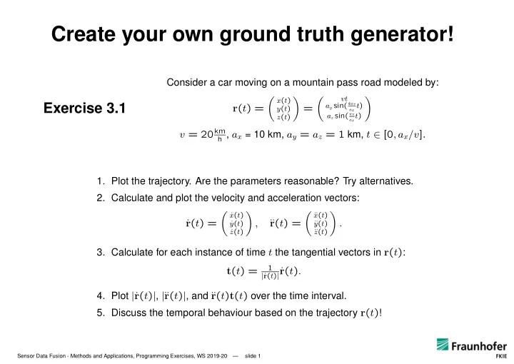
Create your own ground truth generator! Consider a car moving on a mountain pass road modeled by: vt � � � � x ( t ) a y sin( 4 πv Exercise 3.1 ax t ) r ( t ) = = y ( t ) a z sin( πv ax t ) z ( t ) v = 20 km h , a x = 10 km, a y = a z = 1 km, t ∈ [0 , a x /v ] . 1. Plot the trajectory. Are the parameters reasonable? Try alternatives. 2. Calculate and plot the velocity and acceleration vectors: � � � � x ( t ) ˙ x ( t ) ¨ r ( t ) = ˙ , ¨ r ( t ) = . y ( t ) ˙ ¨ y ( t ) z ( t ) ˙ z ( t ) ¨ 3. Calculate for each instance of time t the tangential vectors in r ( t ) : 1 t ( t ) = r ( t ) | ˙ r ( t ) . | ˙ 4. Plot | ˙ r ( t ) | , | ¨ r ( t ) | , and ¨ r ( t ) t ( t ) over the time interval. 5. Discuss the temporal behaviour based on the trajectory r ( t ) ! Sensor Data Fusion - Methods and Applications, Programming Exercises, WS 2019-20 — slide 1

Create your own sensor simulator! Simulate normally distributed radar measurements! ∆ T = 2 s, 2 radars at r 1 , 2 = ( x 1 , 2 s , y 1 , 2 , z 1 , 2 ) ⊤ , s s s Exercise 4.1 x 1 , 2 = 0, 100 km, y 1 , 2 = 100, 0 km, z 1 , 2 = 10 km. s s s State at time t k = k ∆ T , k ∈ Z : x k = ( r ⊤ r ⊤ k ) ⊤ k , ˙ 1. Simulate range and azimuth measurements of the target position r k with a random num- ber generator normrnd (0 , 1) producing normally distributed zero-mean and unit-variance random numbers: � √ � � � ( x k − x s ) 2 +( y k − y s ) 2 +( z k − z s ) 2 − z 2 � � z r z p σ r normrnd (0 , 1) k = = s + k z ϕ yk − ys σ ϕ normrnd (0 , 1) arctan( xk − xs ) k with σ r = 10 m, σ ϕ = 0 . 1 ◦ denoting the standard deviations in range and azimuth. As- sume that the radars are not able to measure the elevation angle (see discussion on the whiteboard!). k ) ⊤ + r s and k (cos z ϕ k , sin z ϕ 2. Transform the measurements in x - y -Cartesian coordinates z r plot them over x - y projection of the true target trajectory! Play with sensor positions and measurement error standard deviations! Sensor Data Fusion - Methods and Applications, Programming Exercises, WS 2019-20 — slide 2

� � p ( x 0 ) = N x 0 ; x 0 | 0 , P 0 | 0 initiation: , initial ignorance: P 0 | 0 ‘large’ dynamics model � � � � N x k − 1 ; x k − 1 | k − 1 , P k − 1 | k − 1 − − − − − − − − − → N x k ; x k | k − 1 , P k | k − 1 prediction: F k | k − 1 , D k | k − 1 x k | k − 1 = F k | k − 1 x k − 1 | k − 1 ⊤ + D k | k − 1 P k | k − 1 = F k | k − 1 P k − 1 | k − 1 F k | k − 1 current measurement z k N � x k ; x k | k − 1 , P k | k − 1 � � � filtering: − − − − − − − − − − − − − → N x k ; x k | k , P k | k sensor model: H k , R k ν k | k − 1 = z k − H k x k | k − 1 x k | k = x k | k − 1 + W k | k − 1 ν k | k − 1 , S k | k − 1 = H k P k | k − 1 H k ⊤ + R k P k | k − 1 − W k | k − 1 S k | k − 1 W k | k − 1 ⊤ , = P k | k W k | k − 1 = P k | k − 1 H k ⊤ S k | k − 1 − 1 ‘K ALMAN gain matrix’ In your sensor simulator, chose a sensor at position r s that produces x - y measurements z k of the Cartesian target x - y positions Hx k from your ground truth generator using the measurement matrix H : � 1 , 0 , 0 , 0 , 0 , 0 � Hx k = x k 0 , 1 , 0 , 0 , 0 , 0 Exercise 4.2 Calculate for each measurement the measurement error covariance matrix R k based on the true target position. Program your first Kalman filter initiated by the first measurement and reasonably chosen covariance matrices P 1 | 1 . What is reasonable? Visualize nicely and compare with the truth and the measurements. Sensor Data Fusion - Methods and Applications, Programming Exercises, WS 2019-20 — slide 3

Selected exercises to be chosen from: Retrodiction — discrete time, eventually continuous time. Simulate missing and false plots — Realize a PDAF tracker. Consider useful IMM parameters — two model IMM tracker. Discretize the road — Realize a road map assisted tracker. Create a GMTI sensor simulator — Realize a GMTI tracker. Test the consistency of one of your trackers — NIS, NEES. Sensor Data Fusion - Methods and Applications, Programming Exercises, WS 2019-20 — slide 4