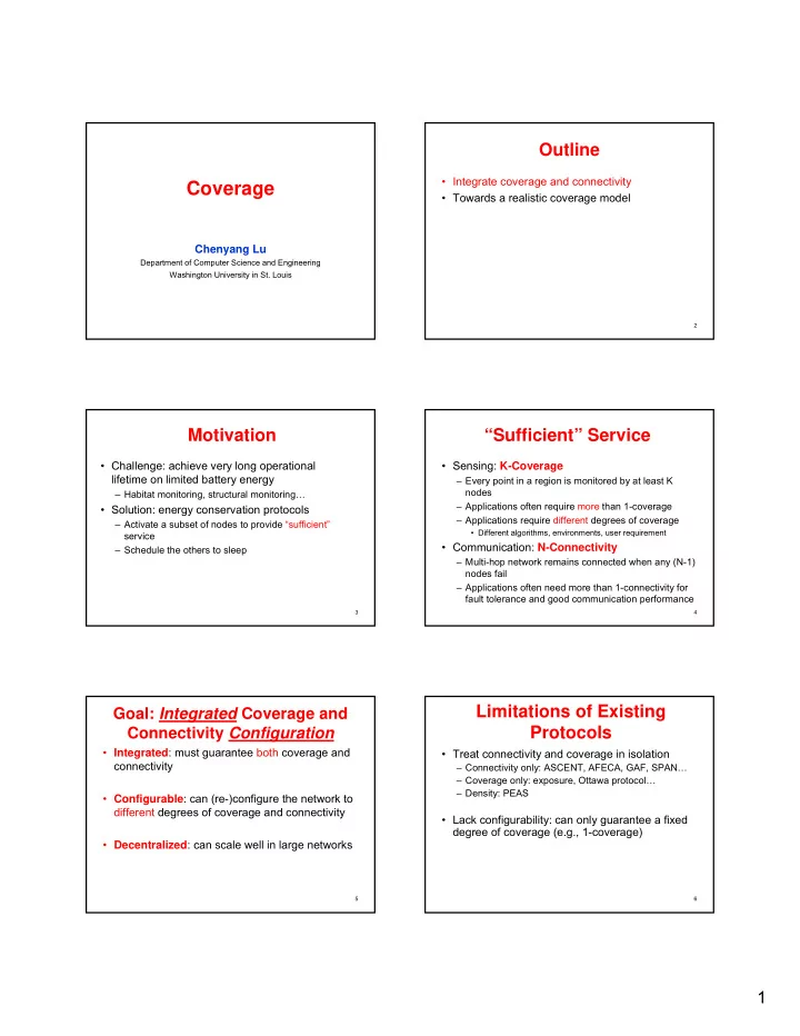
Coverage Towards a realistic coverage model Chenyang Lu - PDF document

Outline • Integrate coverage and connectivity Coverage • Towards a realistic coverage model Chenyang Lu Department of Computer Science and Engineering Washington University in St. Louis 2 Motivation “Sufficient” Service • Challenge: achieve very long operational • Sensing: K-Coverage lifetime on limited battery energy – Every point in a region is monitored by at least K nodes – Habitat monitoring, structural monitoring… – Applications often require more than 1-coverage • Solution: energy conservation protocols – Applications require different degrees of coverage – Activate a subset of nodes to provide “sufficient” • Different algorithms, environments, user requirement service • Communication: N-Connectivity – Schedule the others to sleep – Multi-hop network remains connected when any (N-1) nodes fail – Applications often need more than 1-connectivity for fault tolerance and good communication performance 3 4 Limitations of Existing Goal: Integrated Coverage and Protocols Connectivity Configuration • Integrated : must guarantee both coverage and • Treat connectivity and coverage in isolation connectivity – Connectivity only: ASCENT, AFECA, GAF, SPAN… – Coverage only: exposure, Ottawa protocol… – Density: PEAS • Configurable : can (re-)configure the network to different degrees of coverage and connectivity • Lack configurability: can only guarantee a fixed degree of coverage (e.g., 1-coverage) • Decentralized : can scale well in large networks 5 6 1

Our Approach Assumptions • Disc models for coverage and communication 1. Analyze the geometric relationship between coverage – Point p is covered by node v if |pv| < R s & connectivity • R s : sensing range 2. Design the Coverage Configuration Protocol (CCP) – Nodes u and v are directly connected if |uv| < R c 3. Integrate CCP with SPAN (connectivity maintenance • R c : communication range protocol from MIT) R s • Intuition: R c /R s is important! R c 7 8 Coverage � Connectivity? Connectivity � Coverage? If R c /R s ≥ 2 (the double-range property) • Connectivity cannot guarantee coverage regardless of R c /R s • A covered network is always connected • K -coverage � connectivity ≥ K – Connectivity does not require “connection” with a location with no node • K -coverage � interior connectivity ≥ 2K – Coverage must cover all locations in a region – Interior node: node whose sensing circle locates inside the region – Interior connectivity: number of nodes that must be removed to disconnect any two interior nodes 9 10 Sufficient & Necessary Condition Implication of Analysis for K-Coverage • If R c ≥ 2R s • A region is K-covered iff each intersection point – To achieve K-coverage and N-connectivity, only (between two sensing circles or a sensing circle and the needs to guarantee max(K.N)-coverage region boundary) in the region is K-covered Coverage Configuration Protocol (CCP) is sufficient • Implication: CCP only needs to worry about intersection points! • If R c < 2R s – The protocol must consider both coverage and Every point in a “patch” connectivity. surrounded by sensing Need to integrate CCP with a connectivity circles has the same S maintenance protocol degree of coverage p 11 12 2

CCP: K-Coverage Eligibility Rule CCP: Sleep Listen State Transition • A node is eligible if there exists an intersection point in its sensing Active circle that is not K-covered Needs knowledge about the locations of its sensing neighbors • SLEEP state (active nodes within 2R s ) to assess eligibility – Periodically wake up and enter LISTEN state • Incomplete knowledge about sensing neighbors leads to extra active nodes, but will not cause insufficient coverage • LISTEN state – Receive location beacons and announcements (join/withdraw) – If becomes eligible: enter active state after randomized bidding on? – Otherwise return to SLEEP state • ACTIVE state – Receive location beacons and announcements Active nodes – If becomes ineligible: enter SLEEP state after randomized Sleeping nodes bidding Intersection point 13 14 Coverage Configurability What if R c < 2R s ? Min-500,700,900 Average-500 10 Average-700 • CCP alone does not always guarantee connectivity Achieved Coverage degree Average-900 8 • Solution: CCP + SPAN • Combined eligibility rules 6 – A sleeping node becomes eligible if it is eligible under SPAN or CCP – An active node becomes ineligible only if it is ineligible under 4 both SPAN and CCP 2 0 0 1 2 3 4 5 6 7 Required Coverage degree CCP strictly enforced desired coverage degree! 15 16 Coverage vs R c /R s Coverage & Connectivity (R c /R s = 1.5) Coverage Percentage 1 Coverage Percentage 0.8 0.6 0.4 CCP-2Hop SPAN+CCP-2Hop CCP 0.2 SPAN+CCP SPAN CCP SPAN+CCP SPAN 0 0.5 1 1.5 2 2.5 3 SPAN+CCP is necessary when R c < 2R s R c /R s • CCP and SPAN+CCP always guarantees coverage • SPAN cannot guarantee coverage regardless of R c /R s 17 18 3

Packet Delivery Ratio Summary: Integrated Coverage Packet Delivery Ratio and Connectivity Configuration 1.1 1 • Relationship between coverage and connectivity Packet delivery ratio 0.9 – R c ≥ 2R s : K-coverage � K-connectivity 0.8 0.7 – R c < 2R s : Must worry about both requirements 0.6 0.5 • CCP can efficiently (re-)configure a network to different 0.4 CCP-2Hop degrees of coverage 0.3 SPAN+CCP-2Hop CCP 0.2 SPAN+CCP SPAN 0.1 • CCP+SPAN can maintain both coverage and 0 connectivity when R c < 2R s 0.5 1 1.5 2 2.5 3 R c /R s • CCP successfully delivered all packets when R c /R s > 2 • SPAN+CCP and SPAN had higher deliver ratio than CCP when R c /R s < 2 19 20 Outline • Integrate coverage and connectivity • Towards a realistic coverage model 21 22 Problem Formulation Limitations of Existing Coverage Models • Deterministic Sensing Model Network Topology with • Minimize the number of active sensors – Hard artificial boundary between Sensing Coverage “ sensed ” and “ not sensed ” under the coverage constraint – Fail to capture stochastic nature of – Geographic region A is covered if signals • Ignore sensor fusion ∀ ∈ ≥ β ∧ ≤ α ( ( , ) , ( , ) ) ( ) x y A P x y P D F P D (x,y) – Detection probability of active sensors at point (x,y) P F – False alarm rate 23 24 4

Data Fusion Signal Detection Model • Decide local fusion groups How to compute P D (x,y)? • Sensor observation • Design a set of decision rules in P F < α – Noise: Gaussian distribution with mean 0 a fusion group – Event: Gaussian distribution with mean μ Majority Rule – Single sensor: Likelihood Ratio • Introduce signal decay into detection model Local P F thresholds Test (LRT) is optimal – Observed event signal power decays with distance (2~4 – Fusion center: Majority rule is used LRT power) Local – μ = square root of the target signal power ∑ ∏ ∏ P Di (x,y) = − ( , ) ( 1 ( , )) ( , ) P x y P x y P x y • Signal locality D Di Dj Data Fusion > ∈ ∈ | S | S | | i S j S 1 0 0 1 – Detection performance decreases with distance P D (x,y) S1: sensors with decision 1 – A sensor does not contribute to P D (x,y) if point (x,y) is far O(2 n ) S0: sensors with decision 0 combinations away 25 26 Goals Centralized Coverage Algorithm • Single fusion group • Minimize the number of active sensors to • Fusion center runs a coverage algorithm reduce energy consumption – Uses a greedy strategy to activate sensors • Minimize coverage configuration time – Computes local P F for active sensors • Active sensors perform detection using LRT – Online reconfiguration due to sensor failures based on local P F 27 28 Se-Grid: Coverage Algorithm Centralized Coverage Algorithm based on Separate Grids O(2 n ) n – number of while (P Dmin < β) { • Divide region into multiple grids active sensors Find point p(x,y) with min P D (x,y) • Fusion center in each grid runs Activate the sensor closest to p C ompute local P F thresholds for active sensors the centralized algorithm } • Fusing all sensor decisions at single fusion center – Configuration time is reduced via parallel Ignore signal locality processing High computational cost Data fusion is restricted within each grid � redundant active sensors 29 30 5