Course outline Online decision making 1. Statistical active - PDF document
Active Learning and Optimized Information Gathering Lecture 3 Reinforcement Learning CS 101.2 Andreas Krause Announcements Homework 1: out tomorrow Due Thu Jan 22 Project Proposal due Tue Jan 27 (start soon!) Office hours Come to
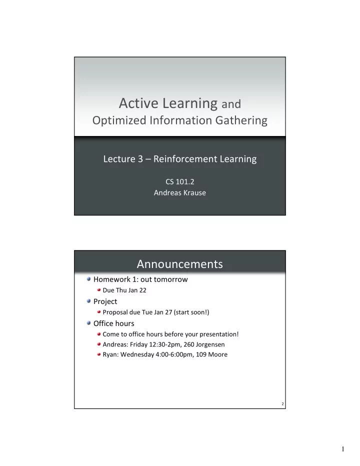
Active Learning and Optimized Information Gathering Lecture 3 – Reinforcement Learning CS 101.2 Andreas Krause Announcements Homework 1: out tomorrow Due Thu Jan 22 Project Proposal due Tue Jan 27 (start soon!) Office hours Come to office hours before your presentation! Andreas: Friday 12:30-2pm, 260 Jorgensen Ryan: Wednesday 4:00-6:00pm, 109 Moore 2 1
Course outline Online decision making 1. Statistical active learning 2. Combinatorial approaches 3. 3 k-armed bandits … p 1 p 2 p 3 p k Each arm i gives reward X i,t with mean µ i 4 2
UCB 1 algorithm: Implicit exploration … p 1 p 2 p 3 p k x Upper conf. Reward Mean µ i Sample avg. 5 UCB 1 algorithm: Implicit exploration … p 1 p 2 p 3 p k x Reward Upper conf. Mean µ i Sample avg. 6 3
UCB 1 algorithm: Implicit exploration … p 1 p 2 p 3 p k Upper conf. Reward Mean µ i Sample avg. 7 Performance of UCB 1 Last lecture: For each suboptimal arm j: E[T j ] = O(log n/ ∆ j ) See notes on course webpage This lecture: What if our actions change the expected reward µ i ?? 8 4
Searching for gold (oil, water, …) S 1 S 2 S 3 S 4 Three actions: • Left • Right • Dig µ Dig µ Dig µ Dig µ Dig µ Left = 0 =0 =0 =.8 =.3 µ Right = 0 x Mean reward depends on internal state! State changes by performing actions 9 Becoming rich and famous 1 (0) ½ (-1) S 1 (-1) poor, poor, ½ (-1) A A unknown famous ½ (0) S ½ (0) ½ (10) ½ (-1) ½ (-1) ½ (10) 1 (-1) S A ½ (10) rich, rich, S A unknown famous ½ (10) 10 5
Markov Decision Processes An MDP has A set of states S = {s 1 ,…,s n } … with reward function r(s,a) [random var. with mean µ s = r(s,a)] A set of actions A = {a 1 ,…,a m } Transition probabilities P(s’|s,a) = Prob(Next state = s’ | Action a in state s) For now assume r and P are known! Want to choose actions to maximize reward Finite horizon Discounted rewards 11 Finite horizon MDP Decision model Reward R = 0 Start in state s For t = 0 to n Choose action a Obtain reward R = R + r(s,a) End up in state s’ according to P(s’|s,a) Repeat with s ← s’ Corresponds to rewards in bandit problems we’ve seen 12 6
Discounted MDP Decision model Reward R = 0 Start in state s For t = 0 to ∞ Choose action a Obtain discounted reward R = R + γ t r(s,a) End up in state s’ according to P(s’|s,a) Repeat with s ← s’ This lecture : Discounted rewards Fixed probability (1- γ ) of “obliteration” (inflation, running out of battery, …) 13 Policies S poor, poor, A A unknown famous S S A rich, rich, S A unknown famous Policy: Pick one fixed action for each state 14 7
Policies: Always save? S poor, poor, unknown famous S S rich, rich, S unknown famous 15 Policies: Always advertise? poor, poor, A A unknown famous A rich, rich, A unknown famous 16 8
Policies: How about this one? poor, poor, A unknown famous S S rich, rich, S unknown famous 17 Planning in MDPs Deterministic policy π : S → A PU PF A Induces a Markov chain : S 1 ,S 2 ,…,S t ,… S S with transition probabilities RU S RF P(S t+1 =s’ | S t =s) = P(s’ | s, π (s)) Expected value J( π ) = E[ r(S 1 , π (S 1 )) + γ r(S 2 , π (S 2 )) + γ 2 r(S 3 , π (S 3 )) + … ] 18 9
Computing the value of a policy For fixed policy π and each state s, define value function V π (s) = J( π | start in state s) = r(s, π (s)) + E[ ∑ t γ t r(S t , π (S t ))] Recursion: and J( π ) = In matrix notation: π analytically, by matrix inversion! ☺ � Can compute V π ☺ ☺ ☺ π π How can we find the optimal policy? 19 A simple algorithm For every policy π compute J( π ) Pick π * = argmax J( π ) Is this a good idea?? 20 10
Value functions and policies Every value function induces a policy Value function V π π π π Greedy policy w.r.t. V V π (s) = r(s, π (s)) + π V (s) = argmax a r(s,a)+ γ ∑ s` P(s’|s, π (s)) V π (s’) γ ∑ s` P(s` | s,a) V(s) Every policy induces a value function Policy optimal � � greedy w.r.t. its induced value function! � � 21 Policy iteration Start with a random policy π Until converged do: Compute value function V π (s) Compute greedy policy π G w.r.t. V π Set π ← π G Guaranteed to Monotonically improve Converge to an optimal policy π * Often performs really well! Not known whether it’s polynomial in |S| and |A|! 22 11
Alternative approach For the optimal policy π * it holds (Bellman equation) V * (s) = max a r(s,a) + γ ∑ s` P(s’ | s ,a) V * (s) Compute V * using dynamic programming: V t (s) = Max. expected reward when starting in state s and world ends in t time steps V 0 (s) = V 1 (s) = V t+1 (s) = 23 Value iteration Initialize V 0 (s) = max a r(s,a) For t = 1 to ∞ For each s, a, let For each s let Break if Then choose greedy policy w.r.t. V t Guaranteed to converge to ε ε ε -optimal policy! ε 24 12
Recap: Ways for solving MDPs Policy iteration: Start with random policy π Compute exact value function V π (matrix inversion) Select greedy policy w.r.t. V π and iterate Value iteration Solve Bellman equation using dynamic programming V t (s) = max a r(s,a) + γ ∑ s` P(s’ | s,a) V t-1 (s) Linear programming 25 MDP = controlled Markov chain A 1 A 2 A t-1 … S 1 S 2 S 3 S t Specify P(S t+1 | S t ,a) State fully observed at every time step Action A t controls transition to S t+1 26 13
POMDP = controlled HMM A 1 A 2 A t-1 … S 1 S 2 S 3 S t O 1 O 2 O 3 O t Specify P(S t+1 | S t ,a t ) P(O t | S t ) Only obtain noisy observations O t of the hidden state S t Very powerful model! ☺ ☺ ☺ ☺ Typically extremely intractable � � � � 27 Applications of MDPs Robot path planning (noisy actions) Elevator scheduling Manufactoring processes Network switching and routing AI in computer games … 28 14
What if the MDP is not known?? ?(?) ? (?) ? (?) S ? (?) poor, poor, ? (?) A ?(?) A unknown famous ? (?) S ? (?) ? (?) ? (?) ? (?) ? (?) S A rich, rich, S A unknown famous ? (?) 29 Bandit problems as unknown MDP 1 (?) 1 Only state 2 1 (?) k … 1 (?) Special case with only 1 state, unknown rewards 30 15
Reinforcement learning World: “You are in state s 17 . You can take actions a 3 and a 9 ” Robot: “I take a 3 ” World: “You get reward -4 and are now in state s 279 . You can take actions a 7 and a 9 ” Robot: “I take a 9 ” World: “You get reward 27 and are now in state s 279 … You can take actions a 2 and a 17 ” … Assumption : States change according to some (unknown) MDP! 31 Credit Assignment Problem State Action Reward S PU PF A A PU A 0 S PU S 0 S A S RU RF A PU A 0 PF S 0 PF A 10 … … … “Wow, I won! How the heck did I do that??” Which actions got me to the state with high reward?? 32 16
Two basic approaches 1) Model-based RL Learn the MDP Estimate transition probabilities P(s’ | s,a) Estimate reward function r(s,a) Optimize policy based on estimated MDP Does not suffer from credit assignment problem! ☺ ☺ ☺ ☺ 2) Model-free RL (later) Estimate the value function directly 33 Exploration–Exploitation Tradeoff in RL We have seen part of the state space and received a reward of 97. S 1 S 2 S 3 S 4 Should we Exploit: stick with our current knowledge and build an optimal policy for the data we’ve seen? Explore: gather more data to avoid missing out on a potentially large reward? 34 17
Possible approaches Always pick a random action? Will eventually converge to optimal policy ☺ Can take very long to find it! � Always pick the best action according to current knowledge? Quickly get some reward Can get stuck in suboptimal action! � 35 Possible approaches ε n greedy With probability ε n : Pick random action With probability (1- ε n ): Pick best action Will converge to optimal policy with probability 1 ☺ Often performs quite well ☺ Doesn’t quickly eliminate clearly suboptimal actions � What about an analogy to UCB1 for bandit problems? 36 18
The R max Algorithm [Brafman & Tennenholz] Optimism in the face of uncertainty! If you don’t know r(s,a): Set it to R max ! If you don’t know P(s’ | s,a): Set P(s* | s,a) = 1 where s* is a “ fairy tale ” state: 37 Implicit Exploration Exploitation in R max Three actions: • Left • Right • Dig r(1,Dig)=0 r(2,Dig)=0 r(3,Dig)=.8 r(4,Dig)=.3 r(i,Left) =0 x r(i,Right)=0 Like UCB1: Never know whether we’re exploring or exploiting! ☺ ☺ ☺ ☺ 38 19
Exploration—Exploitation Lemma Theorem : Every T timesteps, w.h.p., R max either Obtains near-optimal reward, or Visits at least one unknown state-action pair T is related to the mixing time of the Markov chain of the MDP induced by the optimal policy 39 The R max algorithm Input: Starting state s 0 , discount factor γ Initially: Add fairy tale state s * to MDP Set r(s,a) = R max for all states s and actions a Set P(s * | s,a) = 1 for all states s and actions a Repeat: Solve for optimal policy π according to current model P and R Execute policy π For each visited state action pair s, a, update r(s,a) Estimate transition probabilities P(s’ | s,a) If observed “enough” transitions / rewards, recompute policy π 40 20
Recommend
More recommend
Explore More Topics
Stay informed with curated content and fresh updates.
