Cours ENSL: Big Data Streaming, Sketching, Compression Olivier - PowerPoint PPT Presentation
Cours ENSL: Big Data Streaming, Sketching, Compression Olivier Beaumont, Inria Bordeaux Sud-Ouest Olivier.Beaumont@inria.fr 1 Introduction Positionning w.r.t. traditional courses on algorithms Exact algorithms for polynomial
Cours ENSL: Big Data – Streaming, Sketching, Compression Olivier Beaumont, Inria Bordeaux Sud-Ouest Olivier.Beaumont@inria.fr 1
Introduction
Positionning • w.r.t. traditional courses on algorithms • Exact algorithms for polynomial problems • Approximation algorithms for NP-Complete problems • Potentially exponential algorithms for difficult problems (going through an ILP for example) • Here, we will consider extreme contexts • not enough space to transmit input data (sketching) or • not enough space to store the data stream (streaming) • not enough time to use an algorithm other than a linear complexity one • Compared to the more ”classical” context of algorithms: • we aim at solving simple problems and • we are looking for approximate solutions only because we have very strong time or space constraints. • Disclaimer: it is not my research topic, but I like to look at the sketching/streaming papers and I am happy to teach it to you! 2
Application Context 1: Internet of Things (IoT) • Connected objects, which take measurements • The goal is to aggregate data. • Processing can be done either locally, or on their way (fog computing), or in a data center (cloud computing). • We must be very energy efficient • because objects are often embedded without power supply. • E3nergy cost: Communication is the main source of energy consumption, followed by memory movements (from storage), followed by computations (which are inexpensive) • A good solution is to do as many local computations as possible! • but it is known to be difficult (distributed algorithms) • especially when the complexity is not linear (e.g. think about quadratic complexity) • Solution: • compress information locally (and on the fly) • only send the summaries; summaries must contain enough information! 3
Application Context 2: Datacenters • Aggregate construction • except the network (we can have several levels + infiniband), everything is ”linear” • the distance between certain nodes/data is very large but a strong proximity with certain data stored on disk • with 1,000 nodes with 1TB of disk and a link at 400 MB/s, we have 1 PB and 400 GB/s (higher than with a HPC system) • provided the data is loaded locally ! • for 25 TF/s (10 3 25GFs seti@home) in total, ratio 60 (HPC system 40 000) • in practice, dedicated to linear algorithms and very inefficient for other classes. • In both contexts, there is a strong need to have data driven algorithms (where placement is imposed by data) whose complexity is linear 4
Sketching – Streaming
Sketching - Streaming – Context • large volume of data generated in a distributed way • to be processed locally and compressed before transmission. • Types of compression? • lossless compression • compression with losses • compression with losses, but controlled tightly controlled loss for a specific function (sketching) • + we are going to do compression on the fly (streaming) 6
On-the-fly compression dedicated to a function f • Easy problems? • examples: min , max , � , mean value median? • Constraint: linearize the computations (later on plagiarism detection) • How? • The solution is often to switch to randomized approximation algorithms . 7
Compression associated to a specific function f • More formally, given f , • we want to compress the data X but still be able to compute ≃ f ( X ) . • Sketching: we are looking for C f and g such that • the storage space C f ( X ) is small (compression) • from f ( X ), we can recover f ( X ), ie g ( C f ( X )) ≃ f ( X ) • Streaming: additional difficulty, the update is performed on the fly. • we cannot compute C f ( X � { y } ) from X � { y } • since we cannot store X � { y } • so we need another function h such that . h ( C f ( X ) , { y } ) = C f ( X � { y } ) • and one last difficulty: • very often, it is impossible to do in deterministic and exact / deterministic and approximate • but only with a randomized and approximation algorithm. • How to write this ? • We are looking for an estimator Z such that for given α and ǫ • Pr ( | Z − f ( X ) | ≥ ǫ f ( X )) ≤ α . How to read this? • the probability of making a mistake by a ratio greater than ǫ (as small as you want) • is smaller than α (as small as you want) 8
Example: count the number of visits / packets • Context • a sensor/router sees packets / visits passing through,.... • you just want to maintain elementary statistics (number of visits, number of visits over the last 1 hour, standard deviations) • Here, we simply want to count the number of visits • What storage is necessary if we have n visits? log n bits. Why ? Pigeonhole principle. If we have strictly less than logn bits, then we have two events (among the n ) that will be coded in the same way. • What happens if we only allow an approximate answer (say, to a factor of ρ < 2)? you need at least log log n bits. Why ? sketch of the proof: if we use t < log log n bits, then we will be able to distinguish less than log n different groups and you can estimate how many groups are needed to count { 0 } , { 0 , 1 } , { 0 , 1 , 2 } , { 0 , 1 , ..., 7 } . • We will look for a randomized and approximated solution • Let us set α and ǫ • we are looking for an algorithm that computes ˜ n , an approximation of n • that only uses K log log n bits storage • and such that Pr ( | ˜ n − n | ≥ ǫ n ) ≤ α • K must be a constant...not necessarily a small constant for now! 10
Crash Course in probabilities • Z random variable with positive values • E ( Z ) is the expectation of Z • definitions and properties ? • E ( Z ) = � λ P ( Z = λ ) d λ or E ( Z ) = � j jP ( Z = j ) � • E ( Z ) = P ( Z ≥ λ ) d λ or E ( Z ) = � j P ( Z ≥ j ) • E ( aX + bY ) = aE ( X ) + bE ( Y ) • total probabilities (with conditioning) E ( Z ) = � j E ( ZIY = j ) P ( Y = j ) • To measure the distance from Z to E ( Z ), we use the variance V ( Z ) • Definition? • V ( Z ) = E (( Z − E ( Z )) 2 ) = E ( Z 2 ) − E ( Z ) 2 • Properties: • V ( aZ ) = a 2 V ( Z ) • In general, V ( X + Y ) � = V ( X ) + V ( Y ) (but it is true if X and Y are independent random variables) • How to measure the difference between Z to E ( Z )? 1. Markov: Pr ( Z ≥ λ ) ≤ E ( Z ) /λ V ( Z ) 2. Chebyshev: Pr ( | Z − E ( Z ) | ≥ λ E ( Z )) ≤ λ 2 E ( Z ) 2 3. Chernoff: If Z 1 , . . . , Z n are Independent Bernouilli rv with p i ∈ [0 . 1] and Z = � Z i , then Pr ( | Z − E ( Z ) | ≥ λ E ( Z )) ≤ 2 exp( − λ 2 E ( Z ) ). 3 11
Morris Algorithm: Counting the number of events • Step 1: Find an estimator Z • Z must be small (of order of log log n ) • we need to define an additional function g • such that E ( g ( Z )) = n • Morris algorithm • Z → 0 • At each event, Z → Z + 1 with probability 1 / 2 Z • When queried, return f ( Z ) = 2 Z − 1 • What is the space complexity to implement Morris’ algorithm? • What is the time complexity in the worst case? What is the expected complexity of a step? • Prove the correctness: E (2 Z n − 1) = n (note Z n the random variable that denotes Z after n events) Hint: by induction, assuming that E (2 X n ) = n + 1 and showing that E (2 X n +1 ) = n + 2 • How to find a probabilistic guarantee of the type n − n | ≥ ǫ n ) ≤ α ? Hint Prove E (2 2 X n ) = 3 / 2 n 2 + 3 / 2 n + 1. Pr ( | f ( X n ) = ˜ • Conclusion? Is this unexpected ? 12
From Morris to Morris+ and Morris+++ • 2nd step: How to get a useful bound? • Objective: to reduce the variance (expectation is what we want). How to do it? • Classic idea: do the same experience many times and average them • Morris algorithm + • Morris is used to compute independent Z 1 n , Z 2 n , . . . , Z K n i Z i n return f ( Y n ) = 2 Y n − 1 • On demand, compute Y n = � • Questions: • Which space complexity to implement Morris+’s algorithm? • What time complexity? • Establish the correctness: E (2 X n − 1) = n • What is the new guarantee obtained with Chebyshev? How many counters should be maintained? • How can we do even better? • Morris++ = Morris+(1/3) and median • proof with Chernoff: If Z 1 , . . . , Z n are Independent Bernouilli rv with p i ∈ [0 . 1] and Z = � Z i , then Pr ( | Z − E ( Z ) | ≥ λ E ( Z )) ≤ 2 exp( − λ 2 E ( Z ) ). 3 13
2nd example: how to count the number of unique visitors Context • It is assumed that visitors are identified by their address ( i k ∈ [1 , n ]) • We observe a flow of m visits i 1 , . . . , i m with i k ∈ [1 , n ] • How many different visitors ? • Deterministic and trivial algorithms: • if n is small, if n is big... and in front of what? • solution in n : n bit array • solution in m log n : we keep the whole stream! • We will see a bit later • that we cannot do better with exact and deterministic algorithms • that we cannot do better with approximated and deterministic algorithms • How to do if you cannot store n bits • but only O (log k n ) for a certain k ? • we will see that it is again possible by using both randomization and approximation. • and that no deterministic exact or deterministic approximation can do it with this space constraint. 15
Recommend
More recommend
Explore More Topics
Stay informed with curated content and fresh updates.

