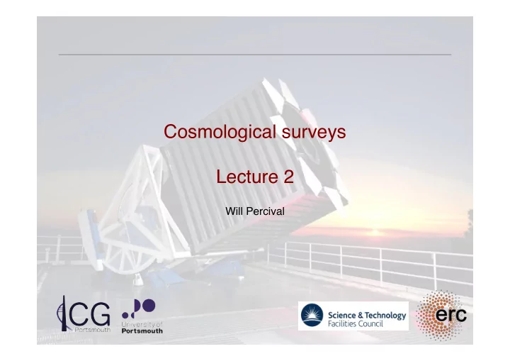
Cosmological surveys Lecture 2 Will Percival " " - PowerPoint PPT Presentation
Cosmological surveys Lecture 2 Will Percival " " Cosmology from surveys " What is the expansion rate of the Universe? " What is the expansion rate of the Understanding " Universe? " Dark Energy " How
Cosmological surveys Lecture 2 Will Percival " "
Cosmology from surveys " What is the expansion rate of the Universe? " What is the expansion rate of the Understanding " Universe? " Dark Energy " How does structure form within Redshift-Space Distortions " Galaxy Survey ! this background? " Weak lensing " What is a combination of the expansion rate of the Universe and the growth rate? " What are the neutrino " Understanding " masses, matter density? " energy-density " What is f nl , which quantifies non- Understanding " Gaussianity? " Inflation "
Weak lensing "
Gravitational lensing " Abell 2218 Cluster of galaxies 2 billion light years away, Background galaxies 6 billion light years away
So what’s happening? "
Weak-lensing " Assumptions: • weak field limit v 2 /c 2 <<1 • stationary field t dyn /t cross <<1 • thin lens approximation L lens /L bench <<1 • transparent lens • small deflection angle
Weak-lensing " Photons travel along null geodesics Solve for photon path by extremizing the Lagrangian for force-free motion L = 1 x µ ˙ x ν 2 g µ ν ˙ This leads to the following Euler-Lagrange equations dp µ dλ = ∂L ∂x µ ; p µ = ∂L ∂ ˙ x µ For the weak-field metric ds 2 = − (1 + 2 Φ ) dt 2 + (1 − 2 Φ ) d x 2 We obtain to first order in ϕ dp ? p − 1 dλ = − 2 r ? Φ ˙ x k k
Weak-lensing " The bend angle depends on the gravitational potential through So the lens equation can be written in terms of a lensing potential The lensing will produce a first order mapping distortion (Jacobian of the lens mapping)
Weak-lensing " We can write the Jacobian of the lens mapping as In terms of the convergence And shear κ represents an isotropic magnification. It transforms a circle into a larger / smaller circle γ Represents an anisotropic magnification. It transforms a circle into an ellipse with axes
Weak-lensing " Galaxy ellipticities provide a direct measurement of the shear field (in the weak lensing limit) Need an expression relating the lensing field to the matter field, which will be an integral over galaxy distances χ The weight function, which depends on the galaxy distribution is The shear power spectra are related to the convergence power spectrum by As expected, from a measurement of the convergence power spectrum we can constrain the matter power spectrum (mainly amplitude) and geometry
Weak-lensing " Comparison of convergence and shear fields "
In practice " • Convergence field can be measured by cross-correlating foreground galaxies with background galaxies " • expect galaxies to be brighter behind mass concentrations • Shear field can be measured from galaxy ellipticities " • percent level e ff ect • requires accurate knowledge of PSF
Intrinsic alignments " • Galaxy formation processes can align galaxies, giving a false shear signal " • correlations can be galaxy-galaxy • correlations can be galaxy-shear • In general, these have a different dependence with redshift compared with the weak lensing signal itself "
Directly depends on the mass distribution " Massey et al. 2008; HST COSMOS analysis; 2 deg 2 !
CFHTLenS " CFHT Lensing Survey: 154deg 2 of deep multi-colour imaging "
CFHTLenS " CFHT Lensing Survey: 154deg 2 of deep multi-colour imaging "
Recent CFHTLenS results " Heymans et al. 2013; arXiv:1303.1808 "
Recent CFHTLenS results " Heymans et al. 2013; arXiv:1303.1808 "
Redshift-space distortions "
Comoving velocities " Locally, galaxies act as test particles in the flow of matter " " On large-scales, the distribution of galaxy velocities is unbiased if galaxies fully sample the velocity field " " expect a small peak velocity-bias due to motion of peaks in Gaussian random fields differing from that of the mass "
Redshift-Space Distortions " When making a 3D map of the Universe the radial distance is usually obtained from a redshift assuming Hubble’s law; this differs from the real-space because of its peculiar velocity: " r − v r ( r ) � r s ( r ) = � � r Where s and r are positions in redshift - and real-space and v r is the peculiar velocity in the radial direction "
Two key regimes of interest " non-linear " linear flow " structure " Actual " Under- Over- Cluster density density shape " Apparent " shape " Under- Over- Cluster density density (viewed from " below) " Power is suppressed " Power is enhanced " on small-scales " on large-scales "
Fingers-of-God clearly visible in maps " Image of SDSS, from U. Chicago "
Linear plane-parallel redshift-space " Transition from real to redshift space, with peculiar velocity v in units of the Hubble flow ! s = r + v los ˆ r los = cos ( α ) µ Jacobian for transformation " θ = ∇ · u μ =0 ◆ 2 ✓ d 3 s ✓ ◆ 1 + v los 1 + dv los d 3 r = r los dr los μ =1 Conservation of galaxy number " n r ( r ) g ) d 3 r ¯ 1 + δ s g = (1 + δ r n r ( r ) d 3 r = n s ( s ) d 3 s n s ( s ) d 3 s ¯ Trick to understand velocity field derivative " ◆ 2 ◆ 2 ✓ ✓ k los ∂ v los ∂ r − 2 θ = θ = µ 2 θ , θ = r · v = ∂ r los ∂ r los k Gives to first order " δ s g = δ r g − µ 2 θ Kaiser 1987, MNRAS, 227, 1 "
what do linear z-space distortions measure? " linear scales, " " = cos ( α ) µ " θ = ∇ · u " " μ =0 " μ =1 Galaxy-galaxy power " Velocity-velocity power " Galaxy-velocity divergence cross power " In linear regime " " δ g = bδ (mass) , θ = − fδ (mass) , f ≡ d ln G " d ln a Linear growth rate " " So, the simplest model for the power spectrum is " " ⇤ 2 P mass ( k ) P s b + µ 2 f ⇥ g ( k, µ ) = " " Kaiser 1987, MNRAS, 227, 1 " "
Modeling redshift space distortions " Include model for both “regimes” " P s P gg ( k ) + 2 µ 2 P g θ ( k ) + µ 4 P θ θ ( k ) F ( k, µ 2 ) ⇥ ⇤ g ( k, µ ) = Note that non-linear model is not necessarily more accurate then the linear one. If we assume linear bias " b 2 + 2 µ 2 fb + µ 4 f 2 ⇤ P s g ( k, µ ) = P r F ( k, µ 2 ) ⇥ m ( k ) On small scales, galaxies lose all knowledge of initial position. If pairwise velocity dispersion has an exponential distribution (superposition of Gaussians), then we get this damping term for the power spectrum. " p / 2) − 1 F ( k, µ 2 ) = (1 + k 2 µ 2 σ 2
Modeling redshift space distortions " Alternative for the data is to try to “correct” the data by “collapsing the clusters” " § Velocity dispersion of the Luminous Red Galaxies (LRGs) shifts them along the line redshift space " of sight by ∼ 9 h − 1 Mpc, and the distribution cylinder " of intrahalo velocities has long tails. " § Use an asymmetric “friends-of- move friends” (FOF) finder to match galaxies in galaxies the same clusters, and collapse to back " spherical profile " § Parameters of FOF calculated by matching simulations " Reid et al. 2008, arXiv:0811.1025; Reid et al. 2009, arXiv:0907.1659 "
Cosmology improved with RSD " • Anisotropic clustering allows huge improvement on w! • w = -0.95 ± 0.25 (WMAP + D V (0.57)/r s ) • w = -0.88 ± 0.055 (WMAP + anisotropic) • Provided a number of GR tests Samushia et al. 2012; arXiv:1206.5309 "
The Alcock-Paczynski Effect "
The Alcock-Paczynski Effect " • If the Universe is isotropic, clustering is same radial & tangential " • Stretching at a single redshift slice (for galaxies expanding with H -1 Universe) depends on " D A H -1 (z) (radial) " D A (z) (angular) " • Analyze with wrong model -> see anisotropy " • AP effect measures D A (z)H(z) " • RSD limits test to scales where can be modeled "
Anisotropic BAO fits … " monopole " quadrupole " Z +1 Z +1 dµ ξ s ( r, µ )3 µ 2 − 1 2 ( r ) = 3 2 ( r ) = 5 ξ s dµ ξ s ( r, µ ) ξ s 2 2 2 − 1 − 1 Anderson et al. 2013; arXiv:1303.4666 "
Anisotropic BAO fits … " • correla'on ¡func'on ¡is ¡easier ¡to ¡split ¡into ¡line-‑of-‑sight ¡and ¡ transverse ¡direc'ons ¡ • can ¡decompose ¡into ¡mul'poles ¡or ¡other ¡bases ¡(e.g. ¡wedges ¡– ¡ see ¡Kazin ¡et ¡al. ¡2013) ¡ • Results ¡are ¡consistent ¡and ¡a ¡concordance ¡value ¡is ¡given ¡ Anderson et al. 2013; arXiv:1303.4666 "
Anisotropic BAO measurements vs CMB " Anderson et al. 2013; arXiv:1303.4666 "
Can we use the AP effect on small scales? " use isolated galaxy pairs ! use voids ! Marinoni & Buzzi 2011 " Lavaux & Wandelt 2011 " Nature 468, 539 " arXiv:1110.0345 " Jennings et al. 2012 " MNRAS 420, 1079 " Both try to isolate objects where the RSD signal is known or weak "
Recommend
More recommend
Explore More Topics
Stay informed with curated content and fresh updates.
