Convex Optimization and Inpainting: A Tutorial Thomas Pock - PowerPoint PPT Presentation
Convex Optimization and Inpainting: A Tutorial Thomas Pock Institute of Computer Graphics and Vision, Graz University of Technology Dagstuhl seminar: Inpainting-Based Image Compression 1 / 56 Shannon-Nyquist sampling theorem In the field of
Convex Optimization and Inpainting: A Tutorial Thomas Pock Institute of Computer Graphics and Vision, Graz University of Technology Dagstuhl seminar: Inpainting-Based Image Compression 1 / 56
Shannon-Nyquist sampling theorem ◮ In the field of digital signal processing, the sampling theorem is a fundamental bridge between continuous-time signals and discrete-time signals ◮ It establishes a sufficient condition for a sample rate that avoids aliasing f s ≥ 2 f max , where f s is the sampling frequency and f max is the maximal frequency of the signal to be sampled. Example: Aliasing in 8 × undersampled image 2 / 56
Compressed sensing ◮ Compressed sensing (CS) is a signal processing technique for efficiently acquiring and reconstructing a signal ◮ It is based on finding solutions to underdetermined linear systems ◮ The underlying principle is that the sparsity of a signal can be exploited to recover it from far fewer samples than required by the Shannon-Nyquist sampling theorem. (a) Original image (b) Sampling (c) No CS (d) Using CS 3 / 56
Solution of underdeterminded systems ◮ Let us consider the following underdetermined system of equations of the form Ax = b ◮ b is a m × 1 measurement vector ◮ x is the n × 1 unknown signal ◮ A is the m × n basis matrix (dictionary), with m < n , which is of the form � � A = a 1 , . . . , a n , where each a i defines a basis atom. ◮ How can we solve the underdetermined system of equations? 4 / 56
Regularization ◮ Let us consider the regularized problem min x f ( x ) subject to Ax = b ◮ A first simple choice is the squared ℓ 2 distance f ( x ) = � x � 2 2 ◮ The unique solution ˆ x of the problem is then given by x 2 = A T ( AA T ) − 1 b , ˆ which is exactly the pseudo-inverse of A . ◮ The quadratic regularization tries to find a solution ˆ x that has the smallest ℓ 2 norm. 5 / 56
Sparsity ◮ Another form of regularization that received a lot of attention during the last years is based on sparsity ◮ The idea is that the underlying ”dimension” of a signals’ complexity is small if represented in a suitable basis ◮ A simple and intuitive form of sparsity is given by the ℓ 0 (pseudo) norm of a vector x � x � 0 = # { i : x i � = 0 } , and hence � x � 0 < n if x is sparse. ◮ Hence we consider the following problem min x � x � 0 subject to Ax = b , which is known as ”Basis Pursuit” [Chen, Donoho ’94] 6 / 56
Convex relaxation ◮ The previous problem is NP-hard and hence very hard to solve if the degree of sparsity is not very small ◮ A simple idea is to replace the ℓ 0 pseudo norm by its closest convex approximation, which is the ℓ 1 norm: min x � x � 1 subject to Ax = b , ◮ This problem can actually be solved using convex optimization algorithms ◮ Under certain circumstances, the solution of the convex ℓ 1 problem yields the same sparse solution as the solution of the ℓ 0 problem 7 / 56
Noise ◮ In case there is noise in the measurement, we can replace the equality in the constraint by an inequality constraint, leading to � Ax − b � 2 ≤ σ 2 , min x � x � 1 subject to where σ > 0 is an estimate of the noise level. ◮ This problem can equivalently be written as the unconstrained optimization problem x � x � 1 + λ 2 � Ax − b � 2 , min where λ > 0 is a suitable Lagrange multiplier. ◮ This model is known as the ”Lasso” (Least absolute shrinkage and selection operator) [Tibshirani ’96] ◮ The model performs a least squares fit while ensuring that only a few basis atoms are used. 8 / 56
The Lasso model ◮ In statistics, the Lasso model is used to perform linear regression and regularization, order to improve the prediction accuracy of a statistical model ◮ Sparsity in the Lasso model has a nice geometric interpretation why the ℓ 1 norm leads to sparse solutions 3 3 2.5 2.5 2 2 1.5 1.5 x 2 x 2 1 1 0.5 0.5 0 0 -0.5 -0.5 -1 -1 -1 -0.5 0 0.5 1 1.5 2 2.5 3 -1 -0.5 0 0.5 1 1.5 2 2.5 3 x 1 x 1 f ( x ) = �·� 2 f ( x ) = �·� 1 2 9 / 56
Example ◮ The Lasso model can also be interpreted as a model that tries to “synthesize” a given signal b using basis atoms from A . basis atoms of A given signal b synthesized signal Ax 10 / 56
Other sparsity inducing functions Besides the ℓ 1 norm, there are other interesting sparsity inducing functions. Assume x ∈ R m × n �� n ◮ Mixed ℓ 1 , 2 norm: � x � 2 , 1 = � m j =1 | x i , j | 2 | can be used i =1 | to induce sparsity in groups of variables ◮ The nuclear norm � x � ∗ = � min { m , n } σ i ( x ) can be used to i =1 induce sparsity in the singular values of x which in turn imposes a low rank prior on x 11 / 56
Synthesis vs. analysis ◮ A closely related (yet different) problem is obtained by moving the linear operator A to the sparsity inducing function. x � By � 1 + λ 2 � y − b � 2 min 2 ◮ Here, the linear operator B can be interpreted as an operator “analyzing” the signal ◮ The model performs a least squares fit while ensuring that the inner product with a given set of basis atomes in B vanishes most of the time ◮ The most influential models in imaging based on such sparse analysis operators are those based on total variation regularization 12 / 56
Convex optimization 1 In imaging, mainly two classes of optimization problems are dominating ◮ “Smooth plus nonsmooth” min x f ( x ) + g ( x ) , where f ( x ) is a smooth function with Lipschitz continuous gradient and g is a simple convex function, with efficient to compute proximal map ◮ Can be solved with proximal gradient methods [Goldstein ’64], [Nesterov ’83], [Combettes, Wajs ’05)], [Beck, Teboulle ’09] y k = ... � x k +1 = prox τ g ( y k − τ ∇ f ( y k )) 13 / 56
Convex optimization 2 ◮ “Non-smooth with linear operator” min x f ( Kx ) + g ( x ) , where f , g are prox-simple convex functions and K is a linear operator ◮ Perform splitting min x , z f ( z ) + g ( x ) , s.t. Kx = z ◮ Consider the augmented Lagrangian � Kx − z , y � + f ( z ) + g ( x ) + 1 2 δ � Kx − z � 2 min x , z max y ◮ Alternating direction of multipliers (ADMM) [Glowinski, Marroco (1975)], [Boyd, Eckstein et al. ’11] ◮ Equivalent to Douglas Rachford splitting [Douglas, Rachford ’56], [Lions, Mercier ’79] ◮ Many variants exist ... 14 / 56
The ROF model ◮ Introduced in [Rudin, Osher, Fatemi ’92] and extended in [Chambolle, Lions ’97] � | Du | + 1 � | u ( x ) − u ⋄ ( x ) | 2 d x , min u λ 2 Ω Ω where Ω is the image domain, u ⋄ is a given (noisy) image and λ > 0 is a regularization parameter. ◮ The term � Ω | Du | is the total variation (TV) of the image u and the gradient operator D is understood in its distributional sense. ◮ A standard way to define the total variation is by duality: � � | Du | := sup − u ( x ) div ϕ ( x ) d x : Ω Ω ϕ ∈ C ∞ c (Ω; R d ) , | ϕ ( x ) | ∗ ≤ 1 , ∀ x ∈ Ω , where Ω ⊂ R d is a d -dimensional open set. 15 / 56
Functions with bounded variation ◮ The space � � � u ∈ L 1 (Ω) : BV(Ω) = | Du | < + ∞ , Ω of functions with bounded variations equipped with the norm � � u � BV = � u � L 1 + Ω | Du | , is a Banach space. ◮ The function | · | could be any norm and the dual norm is given by | φ | ∗ := sup � φ, x � | x |≤ 1 ◮ For smooth images, the TV measures the L 1 norm of the image gradient ◮ The TV is also well-defined for functions with sharp discontinuities ◮ For characteristic functions of smooth sets, it measures exactly the length or area of the surface of the set inside Ω. 16 / 56
Finite differences discretization ◮ In the discrete setting, we consider a scalar-valued digital image u ∈ R m × n of m × n pixels ◮ A simple and standard approach to define the discrete total variation is to define a finite differences operator D : R m × n → R m × n × 2 � u i +1 , j − u i , j if 1 ≤ i < m , ( D u ) i , j , 1 = 0 else , � u i , j +1 − u i , j if 1 ≤ j < n , ( D u ) i , j , 2 = 0 else . ◮ We will also need the operator norm � D � which is estimated as √ � D � ≤ 8 17 / 56
The discrete total variation ◮ The discrete total variation is defined as m , n m , n � 1 / p , � � ( D u ) p i , j , 1 +( D u ) p � � D u � p , 1 = | ( D u ) i , j | p = i , j , 2 i =1 , j =1 i =1 , j =1 that is, the ℓ 1 -norm of the p -norm of the pixelwise image gradients. ◮ For p = 1 we obtain the anisotropic total variation and if p = 2 we obtain the isotropic total variation 18 / 56
Some properties of the total variation ◮ From a sparsity point of view, the total variation induces sparsity in the gradients of the image, hence, it favors piecewise constant images ◮ This property is known as staircasing effect, which is often considered as a drawback for certain applications ◮ The case p = 1 allows for quite effective splitting techniques but favors edges to be aligned with the grid ◮ The case p = 2 can also be considered as a simple form of group sparsity, grouping together the spatial derivatives in each dimension ◮ The isotropic variant does not exhibit a grid bias and hence is often preferred in practice 19 / 56
Recommend
More recommend
Explore More Topics
Stay informed with curated content and fresh updates.
