
Computing Singularity Dimension Mark Pollicott 12 December 2012 1 - PowerPoint PPT Presentation
Introduction Self similar and self-affine sets Hausdorff Dimension Main Theorem Computing Singularity Dimension Mark Pollicott 12 December 2012 1 / 27 Introduction Self similar and self-affine sets Overview Hausdorff Dimension A general
Introduction Self similar and self-affine sets Hausdorff Dimension Main Theorem Computing Singularity Dimension Mark Pollicott 12 December 2012 1 / 27
Introduction Self similar and self-affine sets Overview Hausdorff Dimension A general question Main Theorem Overview In this talk I want to do three things: Recall some familiar examples (which everybody knows); 1 Describe some classic results of Falconer and Hueter-Lalley (which everyone who 2 knows them likes); Present a result on estimating Hausdorff Dimension (which at least I like). 3 2 / 27
Introduction Self similar and self-affine sets Overview Hausdorff Dimension A general question Main Theorem General question Assume that we given some compact set X ⊂ R 2 in the plane. Basic Question What is the Hausdorff Dimension dim H ( X ) of the set X ? Even for the most regular of fractals it can be impossible to give an explicit closed form for the Hausdorff Dimension. A More Practical Question How do we estimate its Hausdorff Dimension dim H ( X )? How well can we approximate dim H ( X )? 3 / 27
Introduction self-similar sets Self similar and self-affine sets Examples of self-similar sets Hausdorff Dimension Self-affine sets Main Theorem Examples of self-affine sets Self-similar sets We call maps T i : R 2 → R 2 ( i = 1 , · · · , k ) of the plane (contracting) similarities if „ a i cos θ i „ x « « „ x « „ b 1 « a i sin θ i T i = + y − a i sin θ i a i cos θ i y b 2 where 0 ≤ θ i < 2 π and 0 < a i < 1 and b 1 , b 2 ∈ R , i.e., rotate by θ i , 1 scale down by a i , and 2 „ b 1 « translate by . 3 b 2 Definition We call a set X ⊂ R 2 self-similar if there are similarities T 1 , · · · , T k : R 2 → R 2 such that T 1 ( X ) ∪ · · · ∪ T k ( X ) = X Self-similar sets are particularly nice to deal with (especially if they also satisfy some extra conditions, e.g., open set condition, strong separation condition, etc). 4 / 27
Introduction self-similar sets Self similar and self-affine sets Examples of self-similar sets Hausdorff Dimension Self-affine sets Main Theorem Examples of self-affine sets Self-similar sets Some examples of self-similar sets have simple expressions for their dimension. (i) Middle third Cantor set . Let T 1 ( x , y ) = ( x 3 , y 3 ) and T 2 ( x , y ) = ( x 3 + 2 3 , y 3 ). √ √ 3 , y 3 y + y (ii) von Koch curve . Let T 1 ( x , y ) = ( x 3 ), T 2 ( x , y ) = ( x 3 x 6 ) + ( 1 6 − 6 , 3 , 0), 6 √ √ √ T 3 ( x , y ) = ( x 3 y 3 x + y 6 ) + ( 1 6 ) and T 4 ( x , y ) = ( x 3 3 + 2 3 , y 6 + 6 , − 2 , + 3 ). 6 5 / 27
Introduction self-similar sets Self similar and self-affine sets Examples of self-similar sets Hausdorff Dimension Self-affine sets Main Theorem Examples of self-affine sets Self-affine sets We say T i : R 2 → R 2 ( i = 1 , · · · , k ) are affine if „ x « „ a 11 « „ x « „ b 1 « a 12 T i = + y a 21 a 22 y b 2 (which we assume to be contractions). i.e., „ a 11 « a 12 apply the linear transformation and 1 a 21 a 22 „ b 1 « translate by . 2 b 2 Definition We call a set X self-affine if there are affine maps if T 1 , · · · , T k : R 2 → R 2 such that T 1 ( X ) ∪ · · · ∪ T k ( X ) After self-similar sets, one would hope self-affine sets are the next easiest to deal with. 6 / 27
Introduction self-similar sets Self similar and self-affine sets Examples of self-similar sets Hausdorff Dimension Self-affine sets Main Theorem Examples of self-affine sets Example 1: Barnsley Fern Consider the four affine maps: „ x « „ 0 . 00 « „ x « 0 . 00 T 1 = y 0 . 00 0 . 16 y „ 0 . 85 „ x « « „ x « „ 0 . 00 « 0 . 04 T 2 = + y − 0 . 04 0 . 85 y 1 . 60 „ x « „ 0 . 20 « „ x « „ 0 . 00 « − 0 . 26 T 3 = + y 0 . 23 0 . 22 y 1 . 60 „ x « „ − 0 . 15 « „ x « „ 0 . 00 « 0 . 28 T 4 = + y 0 . 26 0 . 24 y 0 . 44 The limit set is a fern: 7 / 27
Introduction self-similar sets Self similar and self-affine sets Examples of self-similar sets Hausdorff Dimension Self-affine sets Main Theorem Examples of self-affine sets Example 2: Bedford-McMullen sets This is an standard construction of a self-affine set. Consider for simplicity a s particular special case, called the Hironaka curve, which is the limit set of “ x 3 , y ” T 1 ( x , y ) = 2 „ x « 3 + 1 3 , y 2 + 1 T 2 ( x , y ) = 2 „ x « 3 + 2 3 , y T 3 ( x , y ) = 2 In the limit one gets the “Hironaka curve” . These results were contained in the first published paper of Curt McMullen in 1984. 8 / 27
Introduction self-similar sets Self similar and self-affine sets Examples of self-similar sets Hausdorff Dimension Self-affine sets Main Theorem Examples of self-affine sets Aside: Bedford, McMullen and me Tim Bedford was a PhD student of Caroline Series at Warwick, and an exact contemporary of mine. One day, in Warwick in 1984 he told me about some result in his thesis on Hausdorff Dimension. Later that year I met Curt McMullen, then a PhD student of Dennis Sullivan, in the tea room at IHES (France) and he told me about some results he recently obtained on Hausdorff Dimension. They sounded vaguely familiar. I wrote to Bedford who didn’t know about McMullen’s proof of the same results (who immediately panicked since he hadn’t submitted his PhD yet). Bedford wrote to McMullen (who never panics, although he hadn’t submitted his PhD either). McMullen went on to win a Fields medal and has a chair at Harvard, and Bedford is now an Associate Deputy Principal at the University of Strathclyde. 9 / 27
Introduction Evaluating the dimension Self similar and self-affine sets Falconer’s theorem Hausdorff Dimension Singularity dimension Main Theorem Hueter-Lalley theorem Explicit and Implicit expressions Sometimes it is possible to give explicit expressions for the Hausdorff Dimension when the limit set X is particularly simple. Middle third Cantor set (dim H X = log 2 log 3 ) von Koch Curve (dim H X = log 4 log 3 ) Hironaka curve ( dim H X = log 2 (1 + 2 log 3 2 )) Sometimes it is possible to give implicit expressions for the Hausdorff dimension. For some self-similar sets (open set condition, etc.) some self-conformal sets, (e.g., limit sets of Julia sets, via pressure and the dynamical viewpoint) some special affine sets (e.g., Bedford-McMullen sets) Question How can we (implicitly) describe the Hausdorff dimension of typical limit sets for self-affine maps? 10 / 27
Introduction Evaluating the dimension Self similar and self-affine sets Falconer’s theorem Hausdorff Dimension Singularity dimension Main Theorem Hueter-Lalley theorem Matrices and their singular values Let A 1 , · · · , A k ∈ GL (2 , R ) be 2 × 2 matrices. Given n ≥ 1 and i = ( i 1 , · · · , i n ) ∈ { 1 , · · · , k } n we denote the product of matrices A i = A i 1 A i 2 · · · A i n . We denote their singular values α 1 ( A i ) ≥ α 2 ( A i ). These are the major and minor axes of the ellipse which is the image of the unit circle q A ∗ under A i . Equivalently, these are the eigenvalues of the 2 × 2-matrix i A i . (As explained in the talk of Kenneth Falconer.) Definition We denote ( α 1 ( A i ) s if 0 < s ≤ 1 φ s ( A i ) = α 1 ( A i ) α 1 ( A i ) 1 − s if 1 ≤ s < 2 . 11 / 27
Introduction Evaluating the dimension Self similar and self-affine sets Falconer’s theorem Hausdorff Dimension Singularity dimension Main Theorem Hueter-Lalley theorem Singularity dimension of limit sets Let b 1 , · · · , b k ∈ R 2 we vectors and can consider affine maps T i : R 2 → R 2 defined by T i ( x ) = A i x + b i ( i = 1 , · · · , k ). Definition The limit set Λ ⊂ R 2 is the unique smallest closed set such that Λ = T 1 Λ ∪ · · · ∪ T k Λ. Finally, we have the following definition. Definition We define the singularity dimension of Λ by 8 9 ∞ < = X X φ s ( A i ) < + ∞ dim S (Λ) = inf : s > 0 : ; . n =1 | i | = n where for i = ( i 1 , · · · , i n ) ∈ { 1 , · · · , k } n we write | i | = n . 12 / 27
Introduction Evaluating the dimension Self similar and self-affine sets Falconer’s theorem Hausdorff Dimension Singularity dimension Main Theorem Hueter-Lalley theorem Falconer’s theorem We now recall the elegant theorem of Falconer. Theorem (Falconer, Solomyak) Assume that � A 1 � , · · · , � A k � < 1 2 . For a.e. ( b 1 , · · · , b k ) ∈ R 2 k , we have dim H (Λ) = dim S (Λ) . Figure: Three limit sets corresponding to the same affine contractions A 1 , A 2 , A 3 , but different translations b 1 , b 2 , b 3 . As explained in the talks of Esa J¨ arvenp¨ a¨ a, and Pablo Shmerkin and Jonathan Fraser. 13 / 27
Introduction Evaluating the dimension Self similar and self-affine sets Falconer’s theorem Hausdorff Dimension Singularity dimension Main Theorem Hueter-Lalley theorem Kenneth Falconer and Friends Figure: Karoly Simon, M.P. and Kenneth Falconer 14 / 27
Recommend


More recommend
Explore More Topics
Stay informed with curated content and fresh updates.