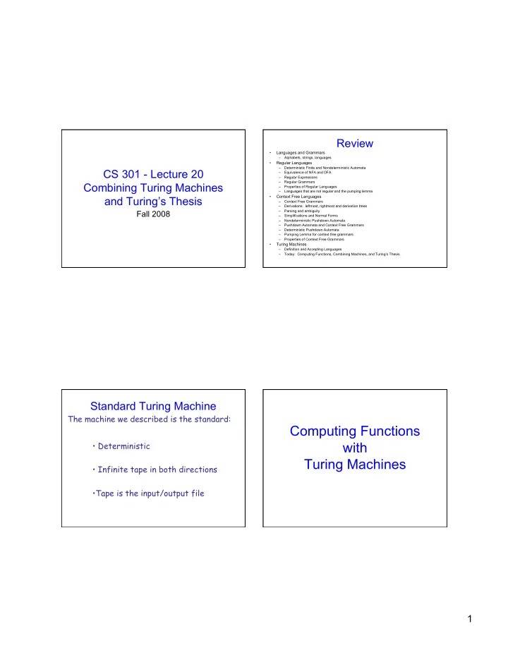

Review • Languages and Grammars – Alphabets, strings, languages • Regular Languages – Deterministic Finite and Nondeterministic Automata CS 301 - Lecture 20 – Equivalence of NFA and DFA – Regular Expressions – Regular Grammars Combining Turing Machines – Properties of Regular Languages – Languages that are not regular and the pumping lemma • Context Free Languages and Turing’s Thesis – Context Free Grammars – Derivations: leftmost, rightmost and derivation trees – Parsing and ambiguity Fall 2008 – Simplifications and Normal Forms – Nondeterministic Pushdown Automata – Pushdown Automata and Context Free Grammars – Deterministic Pushdown Automata – Pumping Lemma for context free grammars – Properties of Context Free Grammars • Turing Machines – Definition and Accepting Languages – Today: Computing Functions, Combining Machines, and Turing’s Thesis Standard Turing Machine The machine we described is the standard: Computing Functions • Deterministic with Turing Machines • Infinite tape in both directions • Tape is the input/output file 1
A function may have many parameters: f ( w ) A function has: Example: Result Region: S Domain: D Addition function f ( x , y ) x y = + f ( w ) f ( w ) S w ∈ D ∈ Definition: Integer Domain f A function is computable if Decimal: 5 M there is a Turing Machine such that: Binary: 101 Initial configuration Final configuration f ( w ) w ◊ ◊ ◊ ◊ Unary: 11111 q q initial state final state f 0 We prefer unary representation: easier to manipulate with Turing machines For all w ∈ D Domain 2
In other words: Example f A function is computable if f ( x , y ) x y The function is computable = + M there is a Turing Machine such that: x , y are integers ∗ q w q f ( w ) 0 f Turing Machine: Initial Final x 0 y Input string: unary Configuration Configuration Output string: xy 0 unary For all w ∈ D Domain y y x x Start Start 1 1 0 1 1 1 1 0 1 1 1 1 ◊ ◊ ◊ ◊ q q initial state 0 0 initial state x + y The 0 is the delimiter that Finish 1 1 1 1 0 ◊ ◊ separates the two numbers q final state f 3
f ( x , y ) x y Turing machine for function = + The 0 helps when we use the result for other operations 1 → 1 , R 1 → 1 , R 1 → 1 , L x + y 0 → 1 , R , L 1 → 0 , L ◊ → ◊ q q q q 2 0 1 3 Finish 1 1 1 1 0 ◊ ◊ , R ◊ → ◊ q q final state f 4 Execution Example: Time 0 Time 0 1 1 0 1 1 ◊ ◊ x y x 11 (2) = 1 1 0 1 1 q ◊ ◊ 0 y 11 (2) = q 0 1 → 1 , R 1 → 1 , R 1 → 1 , L Final Result , L 0 → 1 , R 1 → 0 , L x + y ◊ → ◊ q q q q 2 0 1 3 1 1 1 1 0 ◊ ◊ , R ◊ → ◊ q q 4 4 4
Time 1 Time 2 1 1 0 1 1 1 1 0 1 1 ◊ ◊ ◊ ◊ q q 0 0 1 → 1 , R 1 → 1 , R 1 → 1 , R 1 → 1 , L 1 → 1 , R 1 → 1 , L 0 → 1 , R , L 0 → 1 , R , L 1 → 0 , L 1 → 0 , L ◊ → ◊ ◊ → ◊ q q q q q q q q 2 2 0 1 3 0 1 3 , R , R ◊ → ◊ ◊ → ◊ q q 4 4 Time 3 1 1 1 1 1 Time 4 1 1 1 1 1 ◊ ◊ ◊ ◊ q q 1 1 1 → 1 , R 1 → 1 , R 1 → 1 , R 1 → 1 , L 1 → 1 , R 1 → 1 , L , L , L 0 → 1 , R 1 → 0 , L 0 → 1 , R 1 → 0 , L ◊ → ◊ q ◊ → ◊ q q q q q q q 2 2 0 1 3 0 1 3 , R , R ◊ → ◊ ◊ → ◊ q q 4 4 5
Time 5 Time 6 1 1 1 1 1 1 1 1 1 1 ◊ ◊ ◊ ◊ q q 1 2 1 → 1 , R 1 → 1 , R 1 → 1 , R 1 → 1 , L 1 → 1 , R 1 → 1 , L 0 → 1 , R , L 0 → 1 , R , L 1 → 0 , L 1 → 0 , L ◊ → ◊ ◊ → ◊ q q q q q q q q 2 2 0 1 3 0 1 3 , R , R ◊ → ◊ ◊ → ◊ q q 4 4 Time 7 1 1 1 1 0 Time 8 1 1 1 1 0 ◊ ◊ ◊ ◊ q q 3 3 1 → 1 , R 1 → 1 , R 1 → 1 , R 1 → 1 , L 1 → 1 , R 1 → 1 , L , L , L 0 → 1 , R 1 → 0 , L 0 → 1 , R 1 → 0 , L ◊ → ◊ q ◊ → ◊ q q q q q q q 2 2 0 1 3 0 1 3 , R , R ◊ → ◊ ◊ → ◊ q q 4 4 6
Time 9 0 Time 10 0 1 1 1 1 1 1 1 1 ◊ ◊ ◊ ◊ q q 3 3 1 → 1 , R 1 → 1 , R 1 → 1 , R 1 → 1 , L 1 → 1 , R 1 → 1 , L 0 → 1 , R , L 0 → 1 , R , L 1 → 0 , L 1 → 0 , L ◊ → ◊ ◊ → ◊ q q q q q q q q 2 2 0 1 3 0 1 3 , R , R ◊ → ◊ ◊ → ◊ q q 4 4 Time 11 1 1 1 1 0 Time 12 1 1 1 1 0 ◊ ◊ ◊ ◊ q q 3 4 1 → 1 , R 1 → 1 , R 1 → 1 , R 1 → 1 , L 1 → 1 , R 1 → 1 , L , L , L 0 → 1 , R 1 → 0 , L 0 → 1 , R 1 → 0 , L ◊ → ◊ q ◊ → ◊ q q q q q q q 2 2 0 1 3 0 1 3 , R , R ◊ → ◊ ◊ → ◊ HALT & accept q q 4 4 7
x Another Example f ( x ) 2 x The function is computable = Start 1 1 1 ◊ ◊ x is integer q initial state 0 Turing Machine: 2 x Input string: x unary Finish 1 1 1 1 1 ◊ ◊ xx Output string: unary q final state f f ( x ) 2 x Turing Machine Pseudocode for = f ( x ) 2 x Turing Machine for = • Replace every 1 with $ • Repeat: 1 → $, R 1 → 1 , L 1 → 1 , R • Find rightmost $, replace it with 1 , L $ → 1 , R ◊ → ◊ q • Go to right end, insert 1 q q 2 0 1 , R Until no more $ remain ◊ → ◊ 1 , L ◊ → q 3 8
Example Start Finish Another Example 1 1 ◊ 1 1 1 1 ◊ ◊ ◊ if x > y 1 f ( x , y ) The function = q q 0 3 x ≤ y 0 if is computable 1 → $, R 1 → 1 , L 1 → 1 , R , L $ → 1 , R ◊ → ◊ q q q 2 0 1 , R ◊ → ◊ 1 , L ◊ → q 3 Turing Machine Pseudocode: Turing Machine for • Repeat if x > y 1 f ( x , y ) = y x Match a 1 from with a 1 from x ≤ y 0 if x y Until all of or is matched x 0 y Input: x • If a 1 from is not matched erase tape, write 1 ( x > y ) 1 0 else Output: or erase tape, write 0 ( x ≤ y ) 9
Block Diagram Combining Turing Machines Turing input output Machine Example: x + y if x > y f ( x , y ) = x ≤ y 0 if Turing’s Thesis x , y Adder x + y x > y x , y Comparer x ≤ y 0 Eraser 10
Computer Science Law: A computation is mechanical Turing’s thesis: if and only if it can be performed by a Turing Machine Any computation carried out by mechanical means can be performed by a Turing Machine There is no known model of computation (1930) more powerful than Turing Machines Definition of Algorithm: Algorithms are Turing Machines f ( w ) An algorithm for function is a When we say: Turing Machine which computes f ( w ) There exists an algorithm We mean: There exists a Turing Machine that executes the algorithm 11
What’s Next • Read – Linz Chapter 1,2.1, 2.2, 2.3, (skip 2.4), 3, 4, 5, 6.1, 6.2, (skip 6.3), 7.1, 7.2, 7.3, (skip 7.4), 8, 9, 10.1, 10.2, and 10.3 – JFLAP Chapter 1, 2.1, (skip 2.2), 3, 4, 5, 6, 7, (skip 8), 9 • Next Lecture Topics From 10.1, 10.2 and 10.3 – Turing Machine Variations • Quiz 3 in Recitation on Wednesday 11/12 – Covers Linz 7.1, 7.2, 7.3, (skip 7.4), 8, and JFLAP 5,6,7 – Closed book, but you may bring one sheet of 8.5 x 11 inch paper with any notes you like. – Quiz will take the full hour • Homework – Homework Due Today – New Homework Available Friday Morning – New Homework Due Next Thursday 12
Recommend
More recommend