Computing Absolutely Normal Numbers in Nearly Linear Time Jack H. - PowerPoint PPT Presentation
Computing Absolutely Normal Numbers in Nearly Linear Time Jack H. Lutz and Elvira Mayordomo Iowa State University, Universidad de Zaragoza Continuity, Computability, Constructivity 2017 Loria, Nancy A base is an integer b 2. A base is an
Computing Absolutely Normal Numbers in Nearly Linear Time Jack H. Lutz and Elvira Mayordomo Iowa State University, Universidad de Zaragoza Continuity, Computability, Constructivity 2017 Loria, Nancy
A base is an integer b ≥ 2.
A base is an integer b ≥ 2. A real number α is normal in base b if any two non-empty strings of equal length appear equally often (asymptotically) in the base- b expansion of the fractional part { α } = α mod 1 of α .
A base is an integer b ≥ 2. A real number α is normal in base b if any two non-empty strings of equal length appear equally often (asymptotically) in the base- b expansion of the fractional part { α } = α mod 1 of α . A real number α is absolutely normal if it is normal in every base.
Theorem (Borel, 1909). Almost every real number is absolutely normal.
Theorem (Borel, 1909). Almost every real number is absolutely normal. Theorem (Turing, late 1930s). There is an algorithm that computes an absolutely normal number.
Theorem (Borel, 1909). Almost every real number is absolutely normal. Theorem (Turing, late 1930s). There is an algorithm that computes an absolutely normal number. Theorem (Becher, Heiber, and Slaman, 2013). There is an algorithm that computes an absolutely normal number α in polynomial time. (It computes the successive bits of the binary expansion of α , with the n th bit appearing in time polynomial in n .)
Our result today: An algorithm that computes an absolutely normal number α in nearly linear time.
Our result today: An algorithm that computes an absolutely normal number α in nearly linear time. It computes the successive bits of the binary expansion of α , with the n th bit appearing within n (log n ) O (1) steps.
Our result today: An algorithm that computes an absolutely normal number α in nearly linear time. It computes the successive bits of the binary expansion of α , with the n th bit appearing within n (log n ) O (1) steps. This was called nearly linear time by Gurevich and Shelah (1989), who proved that nearly linear time – unlike linear time! – is model robust.
Outline 1 Martingales (and why) 2 Lempel-Ziv martingales (and why) 3 Savings Accounts 4 Base Change 5 Absolutely Normal Numbers 6 Open Problem (if time)
Martingales Σ b = { 0 , . . . , b − 1 } the base b alphabet Σ ∗ b are finite sequences, Σ ∞ b infinite. sequences x ↾ n is the length- n prefix of x . A martingale is a function d : Σ ∗ b → [0 .. ∞ ) with the fairness property that, for every finite sequence w , � i ∈ Σ b d ( wi ) d ( w ) = . b A martingale d succeeds on an infinite sequence x ∈ Σ ∞ b if limsup n d ( x ↾ n ) = ∞ ( x can be predicted by d ) . Lebesgue measure can be defined in terms of martingales (a set has measure 0 if there is a martingale succeeding on every element of the set). And you have to use martingales to have a useful measure on small complexity classes ... ... because they aggregate a lot of information!
Martingales But how fast do they succeed? Let g : Σ ∗ b → [0 , ∞ ) (may or may not be a martingale) and S ∈ Σ ∞ b . g succeeds on S ( S ∈ S ∞ [ g ]) if lim sup n →∞ g ( S ↾ n ) = ∞ . g f ( n )- succeeds on S ( S ∈ S f ( n ) [ g ]) if log g ( S ↾ n ) lim sup n →∞ > 1. log f ( n ) g succeeds exponentially on S ( S ∈ S exp [ g ]) if ∃ ǫ > 0 S ∈ S 2 ǫ n [ g ].
Lempel-Ziv martingales Schnorr and Stimm (1972) implicitly defined finite-state martingales and proved that every sequence S ∈ Σ ∞ b obeys the following dichotomy: 1 If S is b -normal, then no finite-state base- b martingale succeeds on S . (In fact, every finite-state base- b martingale decays exponentially on S .) 2 If S is not b -normal, then some finite-state base- b martingale succeeds exponentially on S .
Lempel-Ziv martingales Feder (1991) implicitly defined the base- b Lempel-Ziv martingale d LZ ( b ) and proved that it is at least as successful on every sequence as every finite-state martingale.
Lempel-Ziv martingales Feder (1991) implicitly defined the base- b Lempel-Ziv martingale d LZ ( b ) and proved that it is at least as successful on every sequence as every finite-state martingale. b is not normal, then S ∈ S exp [ d LZ ( b ) ]. ∴ if S ∈ Σ ∞
Lempel-Ziv martingales Feder (1991) implicitly defined the base- b Lempel-Ziv martingale d LZ ( b ) and proved that it is at least as successful on every sequence as every finite-state martingale. b is not normal, then S ∈ S exp [ d LZ ( b ) ]. ∴ if S ∈ Σ ∞ ∴ x ∈ (0 , 1) is absolutely normal if none of the martingales d LZ ( b ) succeed exponentially on the base- b expansion of x .
Lempel-Ziv martingales Feder (1991) implicitly defined the base- b Lempel-Ziv martingale d LZ ( b ) and proved that it is at least as successful on every sequence as every finite-state martingale. b is not normal, then S ∈ S exp [ d LZ ( b ) ]. ∴ if S ∈ Σ ∞ ∴ x ∈ (0 , 1) is absolutely normal if none of the martingales d LZ ( b ) succeed exponentially on the base- b expansion of x . Moreover, d LZ ( b ) is fast and has a beautiful theory.
Lempel-Ziv martingales How d LZ ( b ) works: Parse w ∈ Σ ∗ b into distinct phrases , using a growing tree whose leaves are all of the previous phrases. At each step, bet on the next digit in proportion to the number of leaves below each of the b options.
Savings Accounts The value of Lempel-Ziv martingale d LZ ( b ) on a certain infinite string S can fluctuate a lot. This makes base change more complicated (and time consuming). We use the notion of “savings account” here. That is, we construct an alternative martingale that keeps money aside for the bad times to come This is a (refinement of a) technique known since the 1970s.
Savings Accounts The value of Lempel-Ziv martingale d LZ ( b ) on a certain infinite string S can fluctuate a lot. This makes base change more complicated (and time consuming). We use the notion of “savings account” here. That is, we construct an alternative martingale that keeps money aside for the bad times to come This is a (refinement of a) technique known since the 1970s. Definition A savings account for a martingale d : Σ ∗ b → [0 , ∞ ) is a nondecreasing function g : Σ ∗ b → [0 , ∞ ) such that d ( w ) ≥ g ( w ) for every w.
Savings Accounts We construct a new martingale d ′ b with a savings account g ′ b that is a conservative version of d LZ ( b ) . g ′ b succeeds at least on non- b -normal sequences.
Savings Accounts We construct a new martingale d ′ b with a savings account g ′ b that is a conservative version of d LZ ( b ) . g ′ b succeeds at least on non- b -normal sequences. Both d ′ b and g ′ b can be computed in nearly linear time. If S �∈ S ∞ [ g ′ b ] then S is b -normal.
Base Change We want an absolutely normal real number α , that is, the base b representation seq b ( α ) is not in S ∞ [ d ′ b ]. b into a base-2 martingale d (2) For this we convert d ′ b succeeding on the base-2 representations of the reals with base- b representation in S ∞ [ d ′ b ]. Again, d (2) succeeds on seq 2 ( real ( S ∞ [ d ′ b ]). b
Base Change We want an absolutely normal real number α , that is, the base b representation seq b ( α ) is not in S ∞ [ d ′ b ]. b into a base-2 martingale d (2) For this we convert d ′ b succeeding on the base-2 representations of the reals with base- b representation in S ∞ [ d ′ b ]. Again, d (2) succeeds on seq 2 ( real ( S ∞ [ d ′ b ]). b We use Carath´ eodory construction to define measures. Computing in nearly linear time is also delicate.
Base Change We want an absolutely normal real number α , that is, the base b representation seq b ( α ) is not in S ∞ [ d ′ b ]. b into a base-2 martingale d (2) For this we convert d ′ b succeeding on the base-2 representations of the reals with base- b representation in S ∞ [ d ′ b ]. Again, d (2) succeeds on seq 2 ( real ( S ∞ [ d ′ b ]). b We use Carath´ eodory construction to define measures. Computing in nearly linear time is also delicate. In fact our computation � d (2) approximates d (2) slowly b b | � 1 d (2) b ( y ) − d (2) b ( y ) | ≤ | y | 3 .
Absolutely Normal Numbers From previous steps we have a family of martingales ( d (2) b ) b so that d (2) succeeds on base-2 representations of b non- b -normal sequences . For each b we have a nearly linear time computation � d (2) b .
Absolutely Normal Numbers From previous steps we have a family of martingales ( d (2) b ) b so that d (2) succeeds on base-2 representations of b non- b -normal sequences . For each b we have a nearly linear time computation � d (2) b . We want to construct S �∈ S ∞ [ d (2) b ] for every b . Nearly linear time makes it painful to construct a martingale d for the union of S ∞ [ d (2) b ].
Absolutely Normal Numbers From previous steps we have a family of martingales ( d (2) b ) b so that d (2) succeeds on base-2 representations of b non- b -normal sequences . For each b we have a nearly linear time computation � d (2) b . We want to construct S �∈ S ∞ [ d (2) b ] for every b . Nearly linear time makes it painful to construct a martingale d for the union of S ∞ [ d (2) b ]. Then we diagonalize over d to construct S .
Recommend
More recommend
Explore More Topics
Stay informed with curated content and fresh updates.
