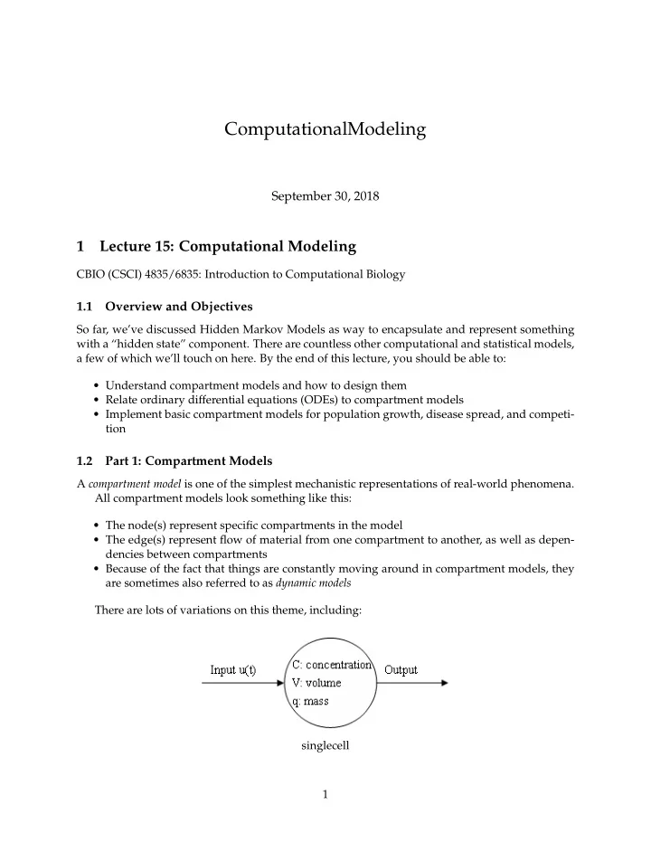

ComputationalModeling September 30, 2018 1 Lecture 15: Computational Modeling CBIO (CSCI) 4835/6835: Introduction to Computational Biology 1.1 Overview and Objectives So far, we’ve discussed Hidden Markov Models as way to encapsulate and represent something with a “hidden state” component. There are countless other computational and statistical models, a few of which we’ll touch on here. By the end of this lecture, you should be able to: • Understand compartment models and how to design them • Relate ordinary differential equations (ODEs) to compartment models • Implement basic compartment models for population growth, disease spread, and competi- tion 1.2 Part 1: Compartment Models A compartment model is one of the simplest mechanistic representations of real-world phenomena. All compartment models look something like this: • The node(s) represent specific compartments in the model • The edge(s) represent flow of material from one compartment to another, as well as depen- dencies between compartments • Because of the fact that things are constantly moving around in compartment models, they are sometimes also referred to as dynamic models There are lots of variations on this theme, including: singlecell 1
singlecell continuous • Closed models : Total amount of material within the model remains constant, simply shifting from one compartment to another • Open models : Total material can flow in and out of the model’s compartments. This is referred to the model having a source (an external contributor of additional material) or a sink (a compartment where material effectively disappears from the model when it enters) • Cyclic models : Material can flow back and forth between mutually connected compart- ments Or combinations of the above! Compartment models can be discrete or continuous . • Discrete models consider the passage of time in discrete steps, e.g. integers. In this example, the input of the compartment u ( t ) is dependent on time, where time is a discrete quantity. • Continuous models , on the other hand, shrink the change in time between events ( δ t ) to 0. We’ll see some examples where this formulation may make more sense. Unfortunately, this is often much more difficult to derive for certain systems. Compartment models can also be deterministic or stochastic . • Deterministic models give you the exact same outputs for any given input. This is what we’ll see with models that use differential equations: for given initial values to the system, we always get the same final values. • Stochastic models introduce randomness into systems, simulating probabilities instead of explicit differential equations. These provide much more realistic looks into real-world sys- tems, but are often much more difficult to analyze (e.g. for steady states), since a given input will not always (or ever!) give the same output. An offshoot of stochastic models is the agent-based model , in which individual “agents” are allowed to act independently according to certain probabilities. This is a very powerful, but very compute-intensive, model. 2
1.3 Part 2: Common Dynamic Models Enough vocabulary; let’s look at a couple common dynamic models. 1.3.1 Population Growth We’d like to model the growth of some population (humans, animals, bacteria, etc). There are two generally-accepted ways of doing this: • Exponential growth assumes that the population grows, well, exponentially. There are im- plicit assumptions here as well, most importantly that resources also grow with population to sustain its growth. • Logistic growth assumes a little more explicitly that the amount of some critical resource (e.g. food) is fixed, effectively providing an upper bound on the ultimate size of the popula- tion. Let’s take a look! Exponential growth sounds a little misleading, since the equation doesn’t, on initial inspec- tion, look exponential. Let’s say your population can grow through birth, and shrink through death. At any given time t , the population is offset by the number added (birth) and removed (death). With this information, can we build an equation for population as a function of time? n ( t + 1 ) = n ( t ) + b − d Or perhaps, put another way, the change in population at any given time? dn dt = bn ( t ) − dn ( t ) • b is the birth rate • d is the death rate • n ( t ) is the population at time t You may notice both terms in the above equation have a common element that can be factored out. dn dt = n ( t )( b − d ) The ( b − d ) term even has a special name: the per capita rate of change . It essentially governs whether the population is increasing or decreasing at any given time, depending on whether the birth or death term dominates. It is typically represented as r c = b − d , so we can rewrite the equation as simply: dn dt = r c n ( t ) Now that we’ve gone through the derivation of the differential equations, how about some nice pretty pictures? Compartment models lend themselves to these sorts of diagrams, which make setting up equa- tions (and, eventually, transition matrices) a lot simpler. So we have these equations; how do we run them and obtain some results? Turns out, Python (specifically, SciPy) has a module for solving ordinary differential equations (ODEs). In [1]: # Preliminary imports %matplotlib inline 3
growthexp import matplotlib.pyplot as plt import numpy as np import scipy.integrate as sig # Here's the critical module! import seaborn as sns Now, let’s set an initial population n 0 , pick a couple of different per capita rates of change r c , and run them to see what happens. In [2]: n0 = 10 rc1 = 0.01 rc2 = 0.1 rc3 = -0.2 The one critical part of the whole thing: you have to define the differential equations as Python functions, so the SciPy module knows what to solve. Let’s do that here: In [3]: # Differential equation functions take two arguments: the variable that's changing, and def diffeq(n, t): return n * rc Now, let’s create a bunch of time points and evaluate the ODE for different values of rc ! In [4]: t = np.linspace(0, 15, 1000) # time rc = rc1 n1, oded = sig.odeint(diffeq, n0, t, full_output = True) print(oded['message']) rc = rc2 n2, oded = sig.odeint(diffeq, n0, t, full_output = True) print(oded['message']) rc = rc3 n3, oded = sig.odeint(diffeq, n0, t, full_output = True) print(oded['message']) 4
Integration successful. Integration successful. Integration successful. In [5]: plt.xlabel('time') plt.ylabel('population') plt.title('Exponential Growth') plt.plot(t, n1, label = '$r_c = 0.01$') plt.plot(t, n2, label = '$r_c = 0.5$') plt.plot(t, n3, label = '$r_c = -0.2$') plt.legend(loc = 0) Out[5]: <matplotlib.legend.Legend at 0x1a1b1108d0> Logistic growth is a slightly different approach. It takes into account the fact that populations usually can’t just keep growing without bound. In fact, their growth rate is directly related to their current size. The model looks something like this: You still see some of the usual suspects–population n ( t ) as a function of time, and birth and death rates, but notice the latter two are also now functions of the current population instead of simply constants. To come up with a bounded model of population growth, we need to add a couple of things to our original equation. 5
growthlog Think of it this way: when the population is small , we want it to behave more or less like it did before–exponential growth. But when the population is large , we want it slow down or even stop growing. dt = r c n ( t )( 1 − n ( t ) dn K ) Let’s look at this more closely: - We still see the same exponential growth equation as before in the first part - There’s a second part, though: ( 1 − n ( t ) K ) - Consider the equation when n ( t ) is small: the n ( t ) K number is close to 0, which means 1 − that number is pretty much 1, so the equation reduces to r c n ( t ) , exactly what we had before! - When n ( t ) is large–say, very close to whatever K is–the fraction n ( t ) is very close to 1, and 1 − 1 = 0, which sets the entire equation to 0. In other K words, growth stops completely! So that’s cool. Let’s plot it out with Python! Remember to first set up the variables and rates: In [6]: # Same as before n0 = 10 rc1 = 0.01 rc2 = 0.1 rc3 = -0.2 K = 100 # The new term introduced by this method--known as "Carrying Capacity" Now we need to write the function that implements the differential equation. In [7]: def logistic_growth(n, t): exp_term = n * rc # same as before limit_term = 1 - (n / K) # the limiting term return exp_term * limit_term Now we simulate it! The only difference is, this time, we feed the function name logistic_growth to the odeint() solver: In [8]: t = np.linspace(0, 100, 2000) # time rc = rc1 n1, oded = sig.odeint(logistic_growth, n0, t, full_output = True) print(oded['message']) 6
rc = rc2 n2, oded = sig.odeint(logistic_growth, n0, t, full_output = True) print(oded['message']) rc = rc3 n3, oded = sig.odeint(logistic_growth, n0, t, full_output = True) print(oded['message']) Integration successful. Integration successful. Integration successful. In [9]: plt.xlabel('time') plt.ylabel('population') plt.title('Logistic Growth with $K = 100$') plt.plot(t, n1, label = '$r_c = 0.01$') plt.plot(t, n2, label = '$r_c = 0.5$') plt.plot(t, n3, label = '$r_c = -0.2$') plt.legend(loc = 0) Out[9]: <matplotlib.legend.Legend at 0x1a1b1c58d0> 7
Recommend
More recommend