Computational Linguistics: Parsing Raffaella Bernardi CIMeC, - PowerPoint PPT Presentation
Computational Linguistics: Parsing Raffaella Bernardi CIMeC, University of Trento e-mail: bernardi@disi.unitn.it Contents First Last Prev Next Contents 1 Done and to be done. . . . . . . . . . . . . . . . . . . . . . . . . . . . . .
4. Kinds of Ambiguities More particularly, in our discussion of parsing we shall be concerned only with two types of ambiguity. ◮ Lexical Ambiguity : a single word can have more than one syntactic category; for example, “smoke” can be a noun or a verb, “her” can be a pronoun or a possessive determiner. ◮ Structural Ambiguity : there are a few valid tree forms for a single sequence of words; for example, which are the possible structures for “old men and women”? It can be grouped either as [[old men] and women] or [old [men and women]]. Contents First Last Prev Next ◭
4.1. Structural Ambiguity An important distinction must also be made between ◮ Global (or total) Ambiguity : in which an entire sentence has several gram- matically allowable analyses. Contents First Last Prev Next ◭
4.1. Structural Ambiguity An important distinction must also be made between ◮ Global (or total) Ambiguity : in which an entire sentence has several gram- matically allowable analyses. ◮ Local (or partial) Ambiguity : in which portions of a sentence, viewed in isolation, may present several possible options, even though the sentence taken as a whole has only one analysis that fits all its parts. Contents First Last Prev Next ◭
4.1. Structural Ambiguity An important distinction must also be made between ◮ Global (or total) Ambiguity : in which an entire sentence has several gram- matically allowable analyses. ◮ Local (or partial) Ambiguity : in which portions of a sentence, viewed in isolation, may present several possible options, even though the sentence taken as a whole has only one analysis that fits all its parts. Contents First Last Prev Next ◭
4.1.1. Global Ambiguity Global ambiguity can be resolved only by resorting to information outside the sentence (the context, etc.) and so cannot be solved by a purely syntactic parser. Contents First Last Prev Next ◭
4.1.1. Global Ambiguity Global ambiguity can be resolved only by resorting to information outside the sentence (the context, etc.) and so cannot be solved by a purely syntactic parser. A good parser should, however, ensure that all possible readings can be found, so that some further disambiguating process could make use of them. Contents First Last Prev Next ◭
4.1.1. Global Ambiguity Global ambiguity can be resolved only by resorting to information outside the sentence (the context, etc.) and so cannot be solved by a purely syntactic parser. A good parser should, however, ensure that all possible readings can be found, so that some further disambiguating process could make use of them. For instance, John saw the woman in the park with the telescope Contents First Last Prev Next ◭
4.1.1. Global Ambiguity Global ambiguity can be resolved only by resorting to information outside the sentence (the context, etc.) and so cannot be solved by a purely syntactic parser. A good parser should, however, ensure that all possible readings can be found, so that some further disambiguating process could make use of them. For instance, John saw the woman in the park with the telescope He was at home. Contents First Last Prev Next ◭
4.1.2. Local Ambiguity Local ambiguity is essentially what makes the orga- nization of a parser non-trivial – the parser may find, in some situations, that the input so far could match more than one of the options that it has (grammatical rules, lexical items, etc). Even if the sentence is not ambiguous as a whole, it may not be possible for the parser to resolve (locally and immediately) which of the possible choices will eventually be correct. “When Fred eats food gets thrown” Contents First Last Prev Next ◭
4.1.2. Local Ambiguity Local ambiguity is essentially what makes the orga- nization of a parser non-trivial – the parser may find, in some situations, that the input so far could match more than one of the options that it has (grammatical rules, lexical items, etc). Even if the sentence is not ambiguous as a whole, it may not be possible for the parser to resolve (locally and immediately) which of the possible choices will eventually be correct. “When Fred eats food gets thrown” ◮ [When Fred eats food] gets thrown?? ◮ [When Fred eats] [food gets thrown] Contents First Last Prev Next ◭
4.1.2. Local Ambiguity Local ambiguity is essentially what makes the orga- nization of a parser non-trivial – the parser may find, in some situations, that the input so far could match more than one of the options that it has (grammatical rules, lexical items, etc). Even if the sentence is not ambiguous as a whole, it may not be possible for the parser to resolve (locally and immediately) which of the possible choices will eventually be correct. “When Fred eats food gets thrown” ◮ [When Fred eats food] gets thrown?? ◮ [When Fred eats] [food gets thrown] Contents First Last Prev Next ◭
4.2. Search Parsing is essentially a search problem (of the kind typically examined in artificial intelligence): Contents First Last Prev Next ◭
4.2. Search Parsing is essentially a search problem (of the kind typically examined in artificial intelligence): ◮ the initial state is the input sequence of words Contents First Last Prev Next ◭
4.2. Search Parsing is essentially a search problem (of the kind typically examined in artificial intelligence): ◮ the initial state is the input sequence of words ◮ the desired final state is a complete tree spanning the whole sentence Contents First Last Prev Next ◭
4.2. Search Parsing is essentially a search problem (of the kind typically examined in artificial intelligence): ◮ the initial state is the input sequence of words ◮ the desired final state is a complete tree spanning the whole sentence ◮ the operators available are the grammar rules and Contents First Last Prev Next ◭
4.2. Search Parsing is essentially a search problem (of the kind typically examined in artificial intelligence): ◮ the initial state is the input sequence of words ◮ the desired final state is a complete tree spanning the whole sentence ◮ the operators available are the grammar rules and ◮ the choices in the search space consist of selecting which rule to apply to which constituents. Contents First Last Prev Next ◭
5. A good Parser A parsing algorithm is provided with a grammar and a string, and it returns possible analyses of that string. Here are the main criteria for evaluating parsing algorithms: Contents First Last Prev Next ◭
5. A good Parser A parsing algorithm is provided with a grammar and a string, and it returns possible analyses of that string. Here are the main criteria for evaluating parsing algorithms: ◮ Correctness : A parser is correct if all the analyses it returns are indeed valid analyses for the string, given the grammar provided. Contents First Last Prev Next ◭
5. A good Parser A parsing algorithm is provided with a grammar and a string, and it returns possible analyses of that string. Here are the main criteria for evaluating parsing algorithms: ◮ Correctness : A parser is correct if all the analyses it returns are indeed valid analyses for the string, given the grammar provided. ◮ Completeness : A parsing algorithm is complete if it returns every possible analysis of every string, given the grammar provided. Contents First Last Prev Next ◭
5. A good Parser A parsing algorithm is provided with a grammar and a string, and it returns possible analyses of that string. Here are the main criteria for evaluating parsing algorithms: ◮ Correctness : A parser is correct if all the analyses it returns are indeed valid analyses for the string, given the grammar provided. ◮ Completeness : A parsing algorithm is complete if it returns every possible analysis of every string, given the grammar provided. ◮ Efficiency : A parsing algorithm should not be unnecessarily complex. For instance, it should not repeat work that only needs to be done once. Contents First Last Prev Next ◭
5.1. Correctness A parser is correct if all the analyses it returns are indeed valid analyses for the string, given the grammar provided . Contents First Last Prev Next ◭
5.1. Correctness A parser is correct if all the analyses it returns are indeed valid analyses for the string, given the grammar provided . ◮ In practice, we almost always require correctness. Contents First Last Prev Next ◭
5.1. Correctness A parser is correct if all the analyses it returns are indeed valid analyses for the string, given the grammar provided . ◮ In practice, we almost always require correctness. ◮ In some cases, however, we might allow the parsing algorithm to produce some analyses that are incorrect , and we would then filter out the bad analyses subsequently. This might be useful if some of the constraints imposed by the grammar were very expensive to test while parsing was in progress but very few possible analyses would actually be rejected by them. Contents First Last Prev Next ◭
5.2. Completeness A parsing algorithm is complete if it returns every possible analysis of every string, given the grammar provided. Contents First Last Prev Next ◭
5.2. Completeness A parsing algorithm is complete if it returns every possible analysis of every string, given the grammar provided. In some circumstances, completeness may not be desirable. For instance, in some applications there may not be time to enumerate all analyses and there may be good heuristics to determine what the “best” analysis is without considering all possibilities. Nevertheless, we will generally assume that the parsing problem entails returning all valid analyses. Contents First Last Prev Next ◭
6. Terminating vs. Complete It is important to realize that there is a distinction between “complete” (i.e. in principle produces all analyses) and “terminating” (i.e. will stop processing in a finite amount of time ). Contents First Last Prev Next ◭
6. Terminating vs. Complete It is important to realize that there is a distinction between “complete” (i.e. in principle produces all analyses) and “terminating” (i.e. will stop processing in a finite amount of time ). A parsing mechanism could be devised which systematically computes every analysis (i.e. is complete) but if it is given a grammar for which there are an infinite number of analyses, it will not terminate. Contents First Last Prev Next ◭
6. Terminating vs. Complete It is important to realize that there is a distinction between “complete” (i.e. in principle produces all analyses) and “terminating” (i.e. will stop processing in a finite amount of time ). A parsing mechanism could be devised which systematically computes every analysis (i.e. is complete) but if it is given a grammar for which there are an infinite number of analyses, it will not terminate. np ---> pn pn ---> np Contents First Last Prev Next ◭
7. Parse Trees: Example Given the grammar: s ---> np vp tv ---> shot np ---> pn pn ---> vincent vp ---> tv np pn ---> marcellus we want to build the parse tree for the sentence “vincent shot marcellus”. Contents First Last Prev Next ◭
7. Parse Trees: Example Given the grammar: s ---> np vp tv ---> shot np ---> pn pn ---> vincent vp ---> tv np pn ---> marcellus we want to build the parse tree for the sentence “vincent shot marcellus”. We know that 1. there must be three leaves and they must be the words “vincent”, “marcellus”, “shot”. Contents First Last Prev Next ◭
7. Parse Trees: Example Given the grammar: s ---> np vp tv ---> shot np ---> pn pn ---> vincent vp ---> tv np pn ---> marcellus we want to build the parse tree for the sentence “vincent shot marcellus”. We know that 1. there must be three leaves and they must be the words “vincent”, “marcellus”, “shot”. 2. the parse tree must have one root, which must be the start symbol s . Contents First Last Prev Next ◭
7. Parse Trees: Example Given the grammar: s ---> np vp tv ---> shot np ---> pn pn ---> vincent vp ---> tv np pn ---> marcellus we want to build the parse tree for the sentence “vincent shot marcellus”. We know that 1. there must be three leaves and they must be the words “vincent”, “marcellus”, “shot”. 2. the parse tree must have one root, which must be the start symbol s . We can now use either the input words or the rules of the grammar to drive the process. Accordingly to the choice we make, we obtain a “bottom up” and “top- down” parsing, respectively. Contents First Last Prev Next ◭
8. Bottom up Parsing The basic idea of bottom up parsing and recognition is: ◮ to begin with the concrete data provided by the input string — that is, the words we have to parse/recognize — and try to build bigger and bigger pieces of structure using this information. Contents First Last Prev Next ◭
8. Bottom up Parsing The basic idea of bottom up parsing and recognition is: ◮ to begin with the concrete data provided by the input string — that is, the words we have to parse/recognize — and try to build bigger and bigger pieces of structure using this information. ◮ Eventually we hope to put all these pieces of structure together in a way that shows that we have found a sentence. Contents First Last Prev Next ◭
8. Bottom up Parsing The basic idea of bottom up parsing and recognition is: ◮ to begin with the concrete data provided by the input string — that is, the words we have to parse/recognize — and try to build bigger and bigger pieces of structure using this information. ◮ Eventually we hope to put all these pieces of structure together in a way that shows that we have found a sentence. Putting it another way, bottom up parsing is about moving from concrete low-level information to more abstract high-level information. Contents First Last Prev Next ◭
8. Bottom up Parsing The basic idea of bottom up parsing and recognition is: ◮ to begin with the concrete data provided by the input string — that is, the words we have to parse/recognize — and try to build bigger and bigger pieces of structure using this information. ◮ Eventually we hope to put all these pieces of structure together in a way that shows that we have found a sentence. Putting it another way, bottom up parsing is about moving from concrete low-level information to more abstract high-level information. This is reflected in a very obvious point about any bottom up algorithm: in bottom up parsing, we use our CFG rules right to left . Contents First Last Prev Next ◭
8.1. A bit more concretely Consider the CFG rule C → P 1 , P 2 , P 3 . Contents First Last Prev Next ◭
8.1. A bit more concretely Consider the CFG rule C → P 1 , P 2 , P 3 . Working bottom up means that we will try to find a P 1 , a P 2 , and a P 3 in the input that are right next to each other. If we find them, we will use this information to conclude that we have found a C . That is, in bottom up parsing, the flow of information is from the right hand side ( P 1 , P 2 , P 3 ) of the rules to the left hand side of the rules ( C ). Contents First Last Prev Next ◭
8.1. A bit more concretely Consider the CFG rule C → P 1 , P 2 , P 3 . Working bottom up means that we will try to find a P 1 , a P 2 , and a P 3 in the input that are right next to each other. If we find them, we will use this information to conclude that we have found a C . That is, in bottom up parsing, the flow of information is from the right hand side ( P 1 , P 2 , P 3 ) of the rules to the left hand side of the rules ( C ). Let’s look at an example of bottom up parsing/recognition start from a linguistics input. Contents First Last Prev Next ◭
8.2. An Example “Vincent shot Marcellus”. Working bottom up, we might do the following. 1. First we go through the string, systematically looking for strings of length 1 that we can rewrite by using our CFG rules in a right to left direction. Contents First Last Prev Next ◭
8.2. An Example “Vincent shot Marcellus”. Working bottom up, we might do the following. 1. First we go through the string, systematically looking for strings of length 1 that we can rewrite by using our CFG rules in a right to left direction. 2. Now, we have the rule pn → vincent , so using this in a right to left direction gives us: pn shot marcellus. Contents First Last Prev Next ◭
8.2. An Example “Vincent shot Marcellus”. Working bottom up, we might do the following. 1. First we go through the string, systematically looking for strings of length 1 that we can rewrite by using our CFG rules in a right to left direction. 2. Now, we have the rule pn → vincent , so using this in a right to left direction gives us: pn shot marcellus. 3. But wait: we also have the rule np → pn , so using this right to left we build: np shot marcellus. Contents First Last Prev Next ◭
8.2. An Example “Vincent shot Marcellus”. Working bottom up, we might do the following. 1. First we go through the string, systematically looking for strings of length 1 that we can rewrite by using our CFG rules in a right to left direction. 2. Now, we have the rule pn → vincent , so using this in a right to left direction gives us: pn shot marcellus. 3. But wait: we also have the rule np → pn , so using this right to left we build: np shot marcellus. 4. We’re still looking for strings of length 1 that we can rewrite using our CFG rules right to left — but we can’t do anything with np . Contents First Last Prev Next ◭
8.2. An Example “Vincent shot Marcellus”. Working bottom up, we might do the following. 1. First we go through the string, systematically looking for strings of length 1 that we can rewrite by using our CFG rules in a right to left direction. 2. Now, we have the rule pn → vincent , so using this in a right to left direction gives us: pn shot marcellus. 3. But wait: we also have the rule np → pn , so using this right to left we build: np shot marcellus. 4. We’re still looking for strings of length 1 that we can rewrite using our CFG rules right to left — but we can’t do anything with np . 5. But we can do something with the second symbol, “shot”. We have the rule tv → shot , and using this right to left yields: np tv marcellus . Contents First Last Prev Next ◭
8.2. An Example “Vincent shot Marcellus”. Working bottom up, we might do the following. 1. First we go through the string, systematically looking for strings of length 1 that we can rewrite by using our CFG rules in a right to left direction. 2. Now, we have the rule pn → vincent , so using this in a right to left direction gives us: pn shot marcellus. 3. But wait: we also have the rule np → pn , so using this right to left we build: np shot marcellus. 4. We’re still looking for strings of length 1 that we can rewrite using our CFG rules right to left — but we can’t do anything with np . 5. But we can do something with the second symbol, “shot”. We have the rule tv → shot , and using this right to left yields: np tv marcellus . Contents First Last Prev Next ◭
6. Can we rewrite tv using a CFG rule right to left? Contents First Last Prev Next ◭
6. Can we rewrite tv using a CFG rule right to left? No — so it’s time to move on and see what we can do with the last symbol, “mar- cellus”. Contents First Last Prev Next ◭
6. Can we rewrite tv using a CFG rule right to left? No — so it’s time to move on and see what we can do with the last symbol, “mar- cellus”. We have the rule pn → marcellus, and this lets us build: np tv pn Contents First Last Prev Next ◭
6. Can we rewrite tv using a CFG rule right to left? No — so it’s time to move on and see what we can do with the last symbol, “mar- cellus”. We have the rule pn → marcellus, and this lets us build: np tv pn 7. We also have the rule np → pn so using this right to left we build: np tv np Contents First Last Prev Next ◭
6. Can we rewrite tv using a CFG rule right to left? No — so it’s time to move on and see what we can do with the last symbol, “mar- cellus”. We have the rule pn → marcellus, and this lets us build: np tv pn 7. We also have the rule np → pn so using this right to left we build: np tv np 8. Are there any more strings of length 1 we can rewrite using our context free rules right to left? Contents First Last Prev Next ◭
6. Can we rewrite tv using a CFG rule right to left? No — so it’s time to move on and see what we can do with the last symbol, “mar- cellus”. We have the rule pn → marcellus, and this lets us build: np tv pn 7. We also have the rule np → pn so using this right to left we build: np tv np 8. Are there any more strings of length 1 we can rewrite using our context free rules right to left? No — we’ve done them all. Contents First Last Prev Next ◭
6. Can we rewrite tv using a CFG rule right to left? No — so it’s time to move on and see what we can do with the last symbol, “mar- cellus”. We have the rule pn → marcellus, and this lets us build: np tv pn 7. We also have the rule np → pn so using this right to left we build: np tv np 8. Are there any more strings of length 1 we can rewrite using our context free rules right to left? No — we’ve done them all. 9. So now we start again at the beginning looking for strings of length 2 that we can rewrite using our CFG rules right to left. And there is one: we have the rule vp → tv np , and this lets us build: np vp Contents First Last Prev Next ◭
6. Can we rewrite tv using a CFG rule right to left? No — so it’s time to move on and see what we can do with the last symbol, “mar- cellus”. We have the rule pn → marcellus, and this lets us build: np tv pn 7. We also have the rule np → pn so using this right to left we build: np tv np 8. Are there any more strings of length 1 we can rewrite using our context free rules right to left? No — we’ve done them all. 9. So now we start again at the beginning looking for strings of length 2 that we can rewrite using our CFG rules right to left. And there is one: we have the rule vp → tv np , and this lets us build: np vp 10. Are there any other strings of length 2 we can rewrite using our CFG rules right to left? Yes — we can now use: s → np vp , we have built: s 11. And this means we are finished. Contents First Last Prev Next ◭
Working bottom up we have succeeded in rewriting our original string of symbols into the symbol s — so we have successfully recognized “Vincent shot Marcellus” as a sentence. Contents First Last Prev Next ◭
8.3. Example Sara wears the new dress pn → sara pn wears the new dress np → pn np wears the new dress tv → wears np tv the new dress det → the np tv det new dress adj → new np tv det adj dress n → dress np tv det adj n n → adj n np tv det n np → det n np tv np vp → tv np np vp s → np vp s Contents First Last Prev Next ◭
8.4. Remarks on Bottom-up A couple of points are worth emphasizing. This is just one of many possible ways of performing a bottom up analysis. All bottom up algorithms use CFG rules right to left — but there are many different ways this can be done. Contents First Last Prev Next ◭
8.4. Remarks on Bottom-up A couple of points are worth emphasizing. This is just one of many possible ways of performing a bottom up analysis. All bottom up algorithms use CFG rules right to left — but there are many different ways this can be done. To give a rather pointless example: we could have designed our algorithm so that it started reading the input in the middle of the string, and then zig-zagged its way to the front and back. And there are many much more serious variations — such as the choice between depth first and breadth first search that we will look at later today. Contents First Last Prev Next ◭
8.4. Remarks on Bottom-up A couple of points are worth emphasizing. This is just one of many possible ways of performing a bottom up analysis. All bottom up algorithms use CFG rules right to left — but there are many different ways this can be done. To give a rather pointless example: we could have designed our algorithm so that it started reading the input in the middle of the string, and then zig-zagged its way to the front and back. And there are many much more serious variations — such as the choice between depth first and breadth first search that we will look at later today. In fact, the algorithm that we used above is crude and inefficient . But it does have one advantage — it is easy to understand. Contents First Last Prev Next ◭
9. Top down Parsing As we have seen, in bottom-up parsing/recognition we start at the most concrete level (the level of words) and try to show that the input string has the abstract structure we are interested in (this usually means showing that it is a sentence). So we use our CFG rules right-to-left. Contents First Last Prev Next ◭
9. Top down Parsing As we have seen, in bottom-up parsing/recognition we start at the most concrete level (the level of words) and try to show that the input string has the abstract structure we are interested in (this usually means showing that it is a sentence). So we use our CFG rules right-to-left. In top-down parsing/recognition we do the reverse. Contents First Last Prev Next ◭
9. Top down Parsing As we have seen, in bottom-up parsing/recognition we start at the most concrete level (the level of words) and try to show that the input string has the abstract structure we are interested in (this usually means showing that it is a sentence). So we use our CFG rules right-to-left. In top-down parsing/recognition we do the reverse. ◮ We start at the most abstract level (the level of sentences) and work down to the most concrete level (the level of words). Contents First Last Prev Next ◭
9. Top down Parsing As we have seen, in bottom-up parsing/recognition we start at the most concrete level (the level of words) and try to show that the input string has the abstract structure we are interested in (this usually means showing that it is a sentence). So we use our CFG rules right-to-left. In top-down parsing/recognition we do the reverse. ◮ We start at the most abstract level (the level of sentences) and work down to the most concrete level (the level of words). ◮ So, given an input string, we start out by assuming that it is a sentence, and then try to prove that it really is one by using the rules left-to-right. Contents First Last Prev Next ◭
9.1. A bit more concretely That works as follows: 1. If we want to prove that the input is of category s and we have the rule s → np vp , then we will try next to prove that the input string consists of a noun phrase followed by a verb phrase. Contents First Last Prev Next ◭
9.1. A bit more concretely That works as follows: 1. If we want to prove that the input is of category s and we have the rule s → np vp , then we will try next to prove that the input string consists of a noun phrase followed by a verb phrase. 2. If we furthermore have the rule np → det n , we try to prove that the input string consists of a determiner followed by a noun and a verb phrase. Contents First Last Prev Next ◭
9.1. A bit more concretely That works as follows: 1. If we want to prove that the input is of category s and we have the rule s → np vp , then we will try next to prove that the input string consists of a noun phrase followed by a verb phrase. 2. If we furthermore have the rule np → det n , we try to prove that the input string consists of a determiner followed by a noun and a verb phrase. That is, we use the rules in a left-to-right fashion to expand the categories that we want to recognize until we have reached categories that match the preterminal symbols corresponding to the words of the input sentence. Contents First Last Prev Next ◭
9.2. An example The left column represents the sequence of categories and words that is arrived at by replacing one of the categories (identical to the left-hand side of the rule in the second column) on the line above by the right-hand side of the rule or by a word that is assigned that category by the lexicon. s s → np vp np vp vp → v np np v np np → det n np v det n n → adj n np v det adj n np → Sara Sara v det adj n v → wears Sara wears det adj n det → the Sara wears the adj n adj → new Sara wears the new n n → dress Sara wears the new dress Contents First Last Prev Next ◭
9.3. Further choices Of course there are lots of choices still to be made. Contents First Last Prev Next ◭
9.3. Further choices Of course there are lots of choices still to be made. ◮ Do we scan the input string from right-to-left, from left-to-right, or zig-zagging out from the middle? Contents First Last Prev Next ◭
9.3. Further choices Of course there are lots of choices still to be made. ◮ Do we scan the input string from right-to-left, from left-to-right, or zig-zagging out from the middle? ◮ In what order should we scan the rules? More interestingly, do we use depth- first or breadth-first search? Contents First Last Prev Next ◭
9.4. Depth first search Depth first search means that whenever there is more than one rule that could be applied at one point, we explore one possibility and only look at the others when this one fails . Let’s look at an example. Contents First Last Prev Next ◭
9.4. Depth first search Depth first search means that whenever there is more than one rule that could be applied at one point, we explore one possibility and only look at the others when this one fails . Let’s look at an example. s ---> np, vp. np ---> pn. vp ---> iv. vp ---> tv, np. lex(vincent,pn). %alternative notation for pn ---> vincent lex(mia,pn). lex(died,iv). lex(loved,tv). lex(shot,tv). The sentence “Mia loved Vincent” is admitted by this grammar. Let’s see how a top-down parser using depth first search would go about showing this. Contents First Last Prev Next ◭
9.4.1. Example Contents First Last Prev Next ◭
9.4.1. Example Contents First Last Prev Next ◭
9.5. Reflections It should be clear why this approach is called top-down: we clearly work from the abstract to the concrete, and we make use of the CFG rules left-to-right . Contents First Last Prev Next ◭
9.5. Reflections It should be clear why this approach is called top-down: we clearly work from the abstract to the concrete, and we make use of the CFG rules left-to-right . Furthermore, it is an example of depth first search because when we were faced with a choice, we selected one alternative, and worked out its consequences. If the choice turned out to be wrong, we backtracked . Contents First Last Prev Next ◭
9.5. Reflections It should be clear why this approach is called top-down: we clearly work from the abstract to the concrete, and we make use of the CFG rules left-to-right . Furthermore, it is an example of depth first search because when we were faced with a choice, we selected one alternative, and worked out its consequences. If the choice turned out to be wrong, we backtracked . For example, above we were faced with a choice of which way to try and build a vp — using an intransitive verb or a transitive verb. Contents First Last Prev Next ◭
9.5. Reflections It should be clear why this approach is called top-down: we clearly work from the abstract to the concrete, and we make use of the CFG rules left-to-right . Furthermore, it is an example of depth first search because when we were faced with a choice, we selected one alternative, and worked out its consequences. If the choice turned out to be wrong, we backtracked . For example, above we were faced with a choice of which way to try and build a vp — using an intransitive verb or a transitive verb. We first tried to do so using an intransitive verb (at state 4) but this didn’t work out (state 5) so we backtracked and tried a transitive analysis (state 4’). This eventually worked out. Contents First Last Prev Next ◭
9.6. Breadth first search The big difference between breadth-first and depth-first search is that in breadth- first search we carry out all possible choices at once , instead of just picking one. Contents First Last Prev Next ◭
9.6. Breadth first search The big difference between breadth-first and depth-first search is that in breadth- first search we carry out all possible choices at once , instead of just picking one. It is useful to imagine that we are working with a big bag containing all the possibilities we should look at — so in what follows I have used set-theoretic braces to indicate this bag. When we start parsing, the bag contains just one item. Contents First Last Prev Next ◭
9.6.1. An example Contents First Last Prev Next ◭
9.6.1. An example The crucial difference occurs at state 4. There we try both ways of building vp at once. At the next step, the intransitive analysis is discarded, but the transitive analysis remains Contents First Last Prev Next ◭
in the bag, and eventually succeeds. Contents First Last Prev Next ◭
9.7. Comparing Depth first and Breadth first searches ◮ The advantage of breadth-first search is that it prevents us from zeroing in on one choice that may turn out to be completely wrong; this often happens with depth-first search, which causes a lot of backtracking. ◮ Its disadvantage is that we need to keep track of all the choices — and if the bag gets big (and it may get very big) we pay a computational price. So which is better? Contents First Last Prev Next ◭
9.7. Comparing Depth first and Breadth first searches ◮ The advantage of breadth-first search is that it prevents us from zeroing in on one choice that may turn out to be completely wrong; this often happens with depth-first search, which causes a lot of backtracking. ◮ Its disadvantage is that we need to keep track of all the choices — and if the bag gets big (and it may get very big) we pay a computational price. So which is better? There is no general answer. With some grammars breadth-first search, with others depth-first. Contents First Last Prev Next ◭
9.8. Exercise Try the two top-down approaches to parse “La vecchia porta sbatte” given the grammar below. det ---> la s --> np vp adj ---> vecchia vp --> iv n ---> vecchia vp --> tv np n ---> porta np --> det n tv ---> porta n --> adj n iv ---> sbatte Contents First Last Prev Next ◭
10. Bottom-up vs. Top-down Parsing Each of these two strategies has its own advantages and disadvantages: Contents First Last Prev Next ◭
10. Bottom-up vs. Top-down Parsing Each of these two strategies has its own advantages and disadvantages: 1. Trees (not) leading to an s Contents First Last Prev Next ◭
Recommend
More recommend
Explore More Topics
Stay informed with curated content and fresh updates.
