Completeness (G odel 1929) Duality proof countermodels : either - PowerPoint PPT Presentation
L UDICS AND LOGICAL COMPLETENESS Geometry of Interaction, Traced Monoidal Categories and Implicit Complexity Workshop, Kyoto, Japan. 28 August 2009 Completeness (G odel 1929) Duality proof countermodels : either there exists a proof
What is ludics? (II) ▶ Monism: An uniform framework in which syntax (proofs) and semantics (counterproofs, models) can be uniformly expressed. ▶ Designs: Untyped paraproofs ▶ “untyped” : proofs from which the logical content has been almost erased. ▶ “para” : proofs which might contain errors and might be incomplete. ▶ Interaction : Designs interact together via normalization which induces an orthogonality relation ⊥ between designs in such a way that P ⊥ M holds if the normalization of P applied to M terminates. ▶ A proof P and “its model” P ⊥ := { N : P ⊥ N } . ▶ An automaton A and a datum D : A accepts D iff A ⊥ D .
What is ludics? (II) ▶ Monism: An uniform framework in which syntax (proofs) and semantics (counterproofs, models) can be uniformly expressed. ▶ Designs: Untyped paraproofs ▶ “untyped” : proofs from which the logical content has been almost erased. ▶ “para” : proofs which might contain errors and might be incomplete. ▶ Interaction : Designs interact together via normalization which induces an orthogonality relation ⊥ between designs in such a way that P ⊥ M holds if the normalization of P applied to M terminates. ▶ A proof P and “its model” P ⊥ := { N : P ⊥ N } . ▶ An automaton A and a datum D : A accepts D iff A ⊥ D .
What is ludics? (II) ▶ Monism: An uniform framework in which syntax (proofs) and semantics (counterproofs, models) can be uniformly expressed. ▶ Designs: Untyped paraproofs ▶ “untyped” : proofs from which the logical content has been almost erased. ▶ “para” : proofs which might contain errors and might be incomplete. ▶ Interaction : Designs interact together via normalization which induces an orthogonality relation ⊥ between designs in such a way that P ⊥ M holds if the normalization of P applied to M terminates. ▶ A proof P and “its model” P ⊥ := { N : P ⊥ N } . ▶ An automaton A and a datum D : A accepts D iff A ⊥ D .
What is ludics? (II) ▶ Monism: An uniform framework in which syntax (proofs) and semantics (counterproofs, models) can be uniformly expressed. ▶ Designs: Untyped paraproofs ▶ “untyped” : proofs from which the logical content has been almost erased. ▶ “para” : proofs which might contain errors and might be incomplete. ▶ Interaction : Designs interact together via normalization which induces an orthogonality relation ⊥ between designs in such a way that P ⊥ M holds if the normalization of P applied to M terminates. ▶ A proof P and “its model” P ⊥ := { N : P ⊥ N } . ▶ An automaton A and a datum D : A accepts D iff A ⊥ D .
What is ludics? (II) ▶ Monism: An uniform framework in which syntax (proofs) and semantics (counterproofs, models) can be uniformly expressed. ▶ Designs: Untyped paraproofs ▶ “untyped” : proofs from which the logical content has been almost erased. ▶ “para” : proofs which might contain errors and might be incomplete. ▶ Interaction : Designs interact together via normalization which induces an orthogonality relation ⊥ between designs in such a way that P ⊥ M holds if the normalization of P applied to M terminates. ▶ A proof P and “its model” P ⊥ := { N : P ⊥ N } . ▶ An automaton A and a datum D : A accepts D iff A ⊥ D .
Example A = n = sssss . . . s 0 풮 OK � �� � start 0 n times s A dialogue between the automata and the datum. 〈 A := x ∣풮 zero . OK + succ ( x ) . A ⟩ 0 := 풮 ( x ) . x ∣ zero 〈 〉 N + 1 := 풮 ( x ) . x ∣ succ N ( ) 풮 ( x ) . x ∣ zero ∣풮⟨ zero . OK + succ ( x ) . A ⟩ A [ 0 / x ] = − → ( zero . OK + succ ( x ) . A ) ∣ zero − → OK . ( ) A [ N + 1 / x ] = 풮 ( x ) . x ∣ succ ⟨ N ⟩ ∣풮⟨ zero . OK + succ ( x ) . A ⟩ ( ) − → zero . OK + succ ( x ) . A ∣ succ ⟨ N ⟩ − → A [ N / x ] .
Example A = n = sssss . . . s 0 풮 OK � �� � start 0 n times s A dialogue between the automata and the datum. 〈 A := x ∣풮 zero . OK + succ ( x ) . A ⟩ 0 := 풮 ( x ) . x ∣ zero 〈 〉 N + 1 := 풮 ( x ) . x ∣ succ N ( ) 풮 ( x ) . x ∣ zero ∣풮⟨ zero . OK + succ ( x ) . A ⟩ A [ 0 / x ] = − → ( zero . OK + succ ( x ) . A ) ∣ zero − → OK . ( ) A [ N + 1 / x ] = 풮 ( x ) . x ∣ succ ⟨ N ⟩ ∣풮⟨ zero . OK + succ ( x ) . A ⟩ ( ) − → zero . OK + succ ( x ) . A ∣ succ ⟨ N ⟩ − → A [ N / x ] .
Example A = n = sssss . . . s 0 풮 OK � �� � start 0 n times s A dialogue between the automata and the datum. 〈 A := x ∣풮 zero . OK + succ ( x ) . A ⟩ 0 := 풮 ( x ) . x ∣ zero 〈 〉 N + 1 := 풮 ( x ) . x ∣ succ N ( ) 풮 ( x ) . x ∣ zero ∣풮⟨ zero . OK + succ ( x ) . A ⟩ A [ 0 / x ] = − → ( zero . OK + succ ( x ) . A ) ∣ zero − → OK . ( ) A [ N + 1 / x ] = 풮 ( x ) . x ∣ succ ⟨ N ⟩ ∣풮⟨ zero . OK + succ ( x ) . A ⟩ ( ) − → zero . OK + succ ( x ) . A ∣ succ ⟨ N ⟩ − → A [ N / x ] .
What is ludics? (III) The core of ludics : focalization Positive Negative ⊗ ` ⊕ & 0 ⊤ 1 ⊥ ? ! ⊢ Σ , A , B ⇕ ▶ Negative = reversible, deterministic: ⊢ Σ , A ` A ⊢ Σ 1 , A ⊢ Σ 2 , B ⇓ ▶ Positive = irreversible, nondeterministic: ⊢ Σ , A ⊗ B
What is ludics? (III) The core of ludics : focalization Positive Negative ⊗ ` ⊕ & 0 ⊤ 1 ⊥ ? ! ⊢ Σ , A , B ⇕ ▶ Negative = reversible, deterministic: ⊢ Σ , A ` A ⊢ Σ 1 , A ⊢ Σ 2 , B ⇓ ▶ Positive = irreversible, nondeterministic: ⊢ Σ , A ⊗ B
What is ludics? (III) The core of ludics : focalization Positive Negative ⊗ ` ⊕ & 0 ⊤ 1 ⊥ ? ! ⊢ Σ , A , B ⇕ ▶ Negative = reversible, deterministic: ⊢ Σ , A ` A ⊢ Σ 1 , A ⊢ Σ 2 , B ⇓ ▶ Positive = irreversible, nondeterministic: ⊢ Σ , A ⊗ B
What is ludics? (III) The core of ludics : focalization Positive Negative ⊗ ` ⊕ & 0 ⊤ 1 ⊥ ? ! ⊢ Σ , A , B ⇕ ▶ Negative = reversible, deterministic: ⊢ Σ , A ` A ⊢ Σ 1 , A ⊢ Σ 2 , B ⇓ ▶ Positive = irreversible, nondeterministic: ⊢ Σ , A ⊗ B
What is ludics? (IV) ▶ ⊢ N 1 , . . . , N m , P 1 , . . . , P n choose a negative formula (if any) and keep decomposing until one get to atoms or positive subformulas; ▶ ⊢ P 1 , . . . , P n choose a positive formula and keep decomposing it up to atoms or negative subformulas. (Andreoli 92) The focalization discipline is a complete proof-search strategy.
What is ludics? (IV) ▶ ⊢ N 1 , . . . , N m , P 1 , . . . , P n choose a negative formula (if any) and keep decomposing until one get to atoms or positive subformulas; ▶ ⊢ P 1 , . . . , P n choose a positive formula and keep decomposing it up to atoms or negative subformulas. (Andreoli 92) The focalization discipline is a complete proof-search strategy.
What is ludics? (V) Synthetic connectives ▶ Focalization allows synthetic connectives: clusters of connectives of the same polarity. ▶ N ⊗ ( M 1 ⊕ M 2 ) can be written as a ⟨ N , M 1 , M 2 ⟩ . Think a as a “generalized” ternary connective ⊗ ( ⊕ ) . ⊢ Σ 2 , M 1 ⊢ Σ 2 , M 2 ⊕ 1 ⊕ 2 Σ 1 , N ⊢ Σ 2 , M 1 ⊕ M 2 ⊗ Σ 1 , N ⊢ Σ 2 , M 1 ⊕ M 2 ⊗ ⊢ Σ , N ⊗ ( M 1 ⊕ M 2 ) ⊢ Σ , N ⊗ ( M 1 ⊕ M 2 ) Σ 1 , N ⊢ Σ 2 , M 1 Σ 1 , N ⊢ Σ 2 , M 2 ⊗⊕ 1 ⊗⊕ 2 ⊢ Σ , N ⊗ ( M 1 ⊕ M 2 ) ⊢ Σ , N ⊗ ( M 1 ⊕ M 2 ) ▶ Alternation of positive and negative layers.
What is ludics? (V) Synthetic connectives ▶ Focalization allows synthetic connectives: clusters of connectives of the same polarity. ▶ N ⊗ ( M 1 ⊕ M 2 ) can be written as a ⟨ N , M 1 , M 2 ⟩ . Think a as a “generalized” ternary connective ⊗ ( ⊕ ) . ⊢ Σ 2 , M 1 ⊢ Σ 2 , M 2 ⊕ 1 ⊕ 2 Σ 1 , N ⊢ Σ 2 , M 1 ⊕ M 2 ⊗ Σ 1 , N ⊢ Σ 2 , M 1 ⊕ M 2 ⊗ ⊢ Σ , N ⊗ ( M 1 ⊕ M 2 ) ⊢ Σ , N ⊗ ( M 1 ⊕ M 2 ) Σ 1 , N ⊢ Σ 2 , M 1 Σ 1 , N ⊢ Σ 2 , M 2 ⊗⊕ 1 ⊗⊕ 2 ⊢ Σ , N ⊗ ( M 1 ⊕ M 2 ) ⊢ Σ , N ⊗ ( M 1 ⊕ M 2 ) ▶ Alternation of positive and negative layers.
What is ludics? (V) Synthetic connectives ▶ Focalization allows synthetic connectives: clusters of connectives of the same polarity. ▶ N ⊗ ( M 1 ⊕ M 2 ) can be written as a ⟨ N , M 1 , M 2 ⟩ . Think a as a “generalized” ternary connective ⊗ ( ⊕ ) . ⊢ Σ 2 , M 1 ⊢ Σ 2 , M 2 ⊕ 1 ⊕ 2 Σ 1 , N ⊢ Σ 2 , M 1 ⊕ M 2 ⊗ Σ 1 , N ⊢ Σ 2 , M 1 ⊕ M 2 ⊗ ⊢ Σ , N ⊗ ( M 1 ⊕ M 2 ) ⊢ Σ , N ⊗ ( M 1 ⊕ M 2 ) Σ 1 , N ⊢ Σ 2 , M 1 Σ 1 , N ⊢ Σ 2 , M 2 ⊗⊕ 1 ⊗⊕ 2 ⊢ Σ , N ⊗ ( M 1 ⊕ M 2 ) ⊢ Σ , N ⊗ ( M 1 ⊕ M 2 ) ▶ Alternation of positive and negative layers.
Computational ludics (I) Designs (Terui 08) ≈ infinitary lambda terms (B¨ ohm trees) + named applications + named and superimposed abstractions. cf. ▶ the ”concrete syntax” (Curien 05) ≈ abstract B¨ ohm trees, ▶ the correspondence with linear 휋 -calculus (Faggian-Piccolo 07). Signature: 풜 = ( A , ar ) A is a set of names, ar : A − → ℕ gives an arity to each name.
Computational ludics (II) The set of designs is coinductively defined by: P ::= ✠ Daimon ∣ Ω Divergence ∣ N 0 ∣ a ⟨ N 1 , . . . , N n ⟩ Application N ::= x Variable ∑ a ( ⃗ ∣ x ) . P a Abstraction ▶ where ar ( a ) = n , ⃗ x = x 1 , . . . , x n ▶ ∑ a ( ⃗ x ) . P a is built from { a ( ⃗ x ) . P a } a ∈ A . Compare it with: P ::= ( N 0 ) N 1 . . . N n x ∣ 휆 x 1 ⋅ ⋅ ⋅ x n . P N ::=
Computational ludics (II) The set of designs is coinductively defined by: P ::= ✠ Daimon ∣ Ω Divergence ∣ N 0 ∣ a ⟨ N 1 , . . . , N n ⟩ Application N ::= x Variable ∑ a ( ⃗ ∣ x ) . P a Abstraction ▶ where ar ( a ) = n , ⃗ x = x 1 , . . . , x n ▶ ∑ a ( ⃗ x ) . P a is built from { a ( ⃗ x ) . P a } a ∈ A . Compare it with: P ::= ( N 0 ) N 1 . . . N n x ∣ 휆 x 1 ⋅ ⋅ ⋅ x n . P N ::=
Reduction ▶ Ω allows partial branching: a ( ⃗ x ) . P + b ( ⃗ y ) . Q := a ( ⃗ x ) . P + b ( ⃗ y ) . Q + c ( ⃗ z ) . Ω + d ( ⃗ z ) . Ω + ⋅ ⋅ ⋅ ▶ Reduction rule: ( ∑ a ( x 1 , . . . , x n ) . P a ) ∣ a ⟨ N 1 , . . . , N n ⟩ − → P a [ N 1 / x 1 , . . . , N n / x n ] . ▶ Compare it with ( 휆 x 1 ⋅ ⋅ ⋅ x n . P ) N 1 ⋅ ⋅ ⋅ N n − → P [ N 1 / x 1 , . . . , N n / x n ]
Reduction ▶ Ω allows partial branching: a ( ⃗ x ) . P + b ( ⃗ y ) . Q := a ( ⃗ x ) . P + b ( ⃗ y ) . Q + c ( ⃗ z ) . Ω + d ( ⃗ z ) . Ω + ⋅ ⋅ ⋅ ▶ Reduction rule: ( ∑ a ( x 1 , . . . , x n ) . P a ) ∣ a ⟨ N 1 , . . . , N n ⟩ − → P a [ N 1 / x 1 , . . . , N n / x n ] . ▶ Compare it with ( 휆 x 1 ⋅ ⋅ ⋅ x n . P ) N 1 ⋅ ⋅ ⋅ N n − → P [ N 1 / x 1 , . . . , N n / x n ]
Reduction ▶ Ω allows partial branching: a ( ⃗ x ) . P + b ( ⃗ y ) . Q := a ( ⃗ x ) . P + b ( ⃗ y ) . Q + c ( ⃗ z ) . Ω + d ( ⃗ z ) . Ω + ⋅ ⋅ ⋅ ▶ Reduction rule: ( ∑ a ( x 1 , . . . , x n ) . P a ) ∣ a ⟨ N 1 , . . . , N n ⟩ − → P a [ N 1 / x 1 , . . . , N n / x n ] . ▶ Compare it with ( 휆 x 1 ⋅ ⋅ ⋅ x n . P ) N 1 ⋅ ⋅ ⋅ N n − → P [ N 1 / x 1 , . . . , N n / x n ]
Orthogonality A positive design P is one of the following forms: x ∣ a ⟨ N 1 , . . . , N n ⟩ Head normal form ( ∑ a ( ⃗ x ) . P a ) ∣ a ⟨ N 1 , . . . , N n ⟩ Cut Daimon ✠ Ω Divergence ▶ Dichotomy: For any closed positive design P , → ∗ ✠ or diverges. P − ▶ Orthogonality: Suppose fv ( P ) ⊆ { x 0 } and fv ( M ) = ∅ . → ∗ ✠ . P ⊥ M ⇐ ⇒ P [ M / x 0 ] − Compare it with: 휋휋 ′ is nilpotent. 휋 ⊥ 휋 ′ ⇐ ⇒
Orthogonality A positive design P is one of the following forms: x ∣ a ⟨ N 1 , . . . , N n ⟩ Head normal form ( ∑ a ( ⃗ x ) . P a ) ∣ a ⟨ N 1 , . . . , N n ⟩ Cut Daimon ✠ Ω Divergence ▶ Dichotomy: For any closed positive design P , → ∗ ✠ or diverges. P − ▶ Orthogonality: Suppose fv ( P ) ⊆ { x 0 } and fv ( M ) = ∅ . → ∗ ✠ . P ⊥ M ⇐ ⇒ P [ M / x 0 ] − Compare it with: 휋휋 ′ is nilpotent. 휋 ⊥ 휋 ′ ⇐ ⇒
Orthogonality A positive design P is one of the following forms: x ∣ a ⟨ N 1 , . . . , N n ⟩ Head normal form ( ∑ a ( ⃗ x ) . P a ) ∣ a ⟨ N 1 , . . . , N n ⟩ Cut Daimon ✠ Ω Divergence ▶ Dichotomy: For any closed positive design P , → ∗ ✠ or diverges. P − ▶ Orthogonality: Suppose fv ( P ) ⊆ { x 0 } and fv ( M ) = ∅ . → ∗ ✠ . P ⊥ M ⇐ ⇒ P [ M / x 0 ] − Compare it with: 휋휋 ′ is nilpotent. 휋 ⊥ 휋 ′ ⇐ ⇒
Orthogonality A positive design P is one of the following forms: x ∣ a ⟨ N 1 , . . . , N n ⟩ Head normal form ( ∑ a ( ⃗ x ) . P a ) ∣ a ⟨ N 1 , . . . , N n ⟩ Cut Daimon ✠ Ω Divergence ▶ Dichotomy: For any closed positive design P , → ∗ ✠ or diverges. P − ▶ Orthogonality: Suppose fv ( P ) ⊆ { x 0 } and fv ( M ) = ∅ . → ∗ ✠ . P ⊥ M ⇐ ⇒ P [ M / x 0 ] − Compare it with: 휋휋 ′ is nilpotent. 휋 ⊥ 휋 ′ ⇐ ⇒
Example: termination A = n = sssss . . . s 0 풮 ✠ � �� � start 0 n times s 〈 A := x ∣풮 zero . ✠ + succ ( x ) . A ⟩ 0 := 풮 ( x ) . x ∣ zero 〈 〉 N + 1 := 풮 ( x ) . x ∣ succ N ( ) A [ 0 / x ] = 풮 ( x ) . x ∣ zero ∣풮⟨ zero . ✠ + succ ( x ) . A ⟩ − → ( zero . ✠ + succ ( x ) . A ) ∣ zero − → ✠ . ( ) A [ N + 1 / x ] = 풮 ( x ) . x ∣ succ ⟨ N ⟩ ∣풮⟨ zero . ✠ + succ ( x ) . A ⟩ ( ) − → zero . ✠ + succ ( x ) . A ∣ succ ⟨ N ⟩ − → A [ N / x ] .
Example: termination A = n = sssss . . . s 0 풮 ✠ � �� � start 0 n times s 〈 A := x ∣풮 zero . ✠ + succ ( x ) . A ⟩ 0 := 풮 ( x ) . x ∣ zero 〈 〉 N + 1 := 풮 ( x ) . x ∣ succ N ( ) A [ 0 / x ] = 풮 ( x ) . x ∣ zero ∣풮⟨ zero . ✠ + succ ( x ) . A ⟩ − → ( zero . ✠ + succ ( x ) . A ) ∣ zero − → ✠ . ( ) A [ N + 1 / x ] = 풮 ( x ) . x ∣ succ ⟨ N ⟩ ∣풮⟨ zero . ✠ + succ ( x ) . A ⟩ ( ) − → zero . ✠ + succ ( x ) . A ∣ succ ⟨ N ⟩ − → A [ N / x ] .
Example: termination A = n = sssss . . . s 0 풮 ✠ � �� � start 0 n times s 〈 A := x ∣풮 zero . ✠ + succ ( x ) . A ⟩ 0 := 풮 ( x ) . x ∣ zero 〈 〉 N + 1 := 풮 ( x ) . x ∣ succ N ( ) A [ 0 / x ] = 풮 ( x ) . x ∣ zero ∣풮⟨ zero . ✠ + succ ( x ) . A ⟩ − → ( zero . ✠ + succ ( x ) . A ) ∣ zero − → ✠ . ( ) A [ N + 1 / x ] = 풮 ( x ) . x ∣ succ ⟨ N ⟩ ∣풮⟨ zero . ✠ + succ ( x ) . A ⟩ ( ) − → zero . ✠ + succ ( x ) . A ∣ succ ⟨ N ⟩ − → A [ N / x ] .
Example: nontermination 〈 〉 P := x ∣ a N N := a ( x ) . P M := b ( y ) . P ( ) 〈 〉 P [ N / x ] = a ( x ) . P ∣ a N − → P [ N / x ] . ( ) 〈 〉 ∣ a P [ M / x ] = b ( x ) . P N − → Ω .
Example: nontermination 〈 〉 P := x ∣ a N N := a ( x ) . P M := b ( y ) . P ( ) 〈 〉 P [ N / x ] = a ( x ) . P ∣ a N − → P [ N / x ] . ( ) 〈 〉 ∣ a P [ M / x ] = b ( x ) . P N − → Ω .
Ludics and Game Semantics Ludics Game Semantics Untyped strategies ( designs ) Typed strategies ⊥⊥ Types ( Behaviours ) Types ( Arenas, Games ) ▶ Game Semantics: All strategies are typed. Types GUARANTEE that strategies compose well. ▶ Ludics : Strategies are untyped (all given on a universal arena) Strategies can ALWAYS interact with each other, and interaction may terminate well ( ⊥ ) or not (deadlock, Ω )
Ludics and Game Semantics Ludics Game Semantics Untyped strategies ( designs ) Typed strategies ⊥⊥ Types ( Behaviours ) Types ( Arenas, Games ) ▶ Game Semantics: All strategies are typed. Types GUARANTEE that strategies compose well. ▶ Ludics : Strategies are untyped (all given on a universal arena) Strategies can ALWAYS interact with each other, and interaction may terminate well ( ⊥ ) or not (deadlock, Ω )
Ludics and Game Semantics Ludics Game Semantics Untyped strategies ( designs ) Typed strategies ⊥⊥ Types ( Behaviours ) Types ( Arenas, Games ) ▶ Game Semantics: All strategies are typed. Types GUARANTEE that strategies compose well. ▶ Ludics : Strategies are untyped (all given on a universal arena) Strategies can ALWAYS interact with each other, and interaction may terminate well ( ⊥ ) or not (deadlock, Ω )
Nondeterminism: why ▶ An interactive account and of contraction — duplication rule: P ( x , y ) ⊢ x : P , y : P P ( z , z ) ⊢ z : P where: ▶ P is a positive logical type; ▶ P ( x , y ) is a positive design with free variables in { x , y } ; ▶ P ( z , z ) is a positive design with free variable z . ▶ Two different readings of the rule: Top Down Contraction : an identification of free variables. Bottom Up Duplication : an arbitrary bi-partition of occurrences of z .
Nondeterminism: why ▶ An interactive account and of contraction — duplication rule: P ( x , y ) ⊢ x : P , y : P P ( z , z ) ⊢ z : P where: ▶ P is a positive logical type; ▶ P ( x , y ) is a positive design with free variables in { x , y } ; ▶ P ( z , z ) is a positive design with free variable z . ▶ Two different readings of the rule: Top Down Contraction : an identification of free variables. Bottom Up Duplication : an arbitrary bi-partition of occurrences of z .
Nondeterminism: why ▶ An interactive account and of contraction — duplication rule: P ( x , y ) ⊢ x : P , y : P P ( z , z ) ⊢ z : P where: ▶ P is a positive logical type; ▶ P ( x , y ) is a positive design with free variables in { x , y } ; ▶ P ( z , z ) is a positive design with free variable z . ▶ Two different readings of the rule: Top Down Contraction : an identification of free variables. Bottom Up Duplication : an arbitrary bi-partition of occurrences of z .
Failure of completeness Write P ∣ = Γ for the interpretation of the sequent P ⊢ Γ . Semantically, we have to show that: = x : P , y : P ⇐ = z : P P ( x , y ) ∣ ⇒ P ( z , z ) ∣ ★ In general, ★ does not hold in a uniform setting.... We need to enlarge the universe of designs. We introduce (universal) nondeterminism.
Failure of completeness Write P ∣ = Γ for the interpretation of the sequent P ⊢ Γ . Semantically, we have to show that: = x : P , y : P ⇐ = z : P P ( x , y ) ∣ ⇒ P ( z , z ) ∣ ★ In general, ★ does not hold in a uniform setting.... We need to enlarge the universe of designs. We introduce (universal) nondeterminism.
Failure of completeness Write P ∣ = Γ for the interpretation of the sequent P ⊢ Γ . Semantically, we have to show that: = x : P , y : P ⇐ = z : P P ( x , y ) ∣ ⇒ P ( z , z ) ∣ ★ In general, ★ does not hold in a uniform setting.... We need to enlarge the universe of designs. We introduce (universal) nondeterminism.
Failure of completeness Write P ∣ = Γ for the interpretation of the sequent P ⊢ Γ . Semantically, we have to show that: = x : P , y : P ⇐ = z : P P ( x , y ) ∣ ⇒ P ( z , z ) ∣ ★ In general, ★ does not hold in a uniform setting.... We need to enlarge the universe of designs. We introduce (universal) nondeterminism.
Failure of completeness Write P ∣ = Γ for the interpretation of the sequent P ⊢ Γ . Semantically, we have to show that: = x : P , y : P ⇐ = z : P P ( x , y ) ∣ ⇒ P ( z , z ) ∣ ★ In general, ★ does not hold in a uniform setting.... We need to enlarge the universe of designs. We introduce (universal) nondeterminism.
Designs Coinductively defined terms given by the following grammar: � � ⋀ P ::= Ω I Q i positive designs N 0 ∣ a ⟨ N 1 , . . . , N n ⟩ Q i ::= predesigns � ∑ a ( ⃗ � N ::= x x ) . P a negative designs ▶ ✠ is now defined as the empty conjunction ⋀ ∅ . ⋀ { i } Q i is simply written as Q i . ▶ A designs is deterministic if in any occurrence of subdesign ⋀ I Q i , I is either empty (and hence ⋀ I Q i = ✠ ) or a singleton.
Designs Coinductively defined terms given by the following grammar: � � ⋀ P ::= Ω I Q i positive designs N 0 ∣ a ⟨ N 1 , . . . , N n ⟩ Q i ::= predesigns � ∑ a ( ⃗ � N ::= x x ) . P a negative designs ▶ ✠ is now defined as the empty conjunction ⋀ ∅ . ⋀ { i } Q i is simply written as Q i . ▶ A designs is deterministic if in any occurrence of subdesign ⋀ I Q i , I is either empty (and hence ⋀ I Q i = ✠ ) or a singleton.
Designs Coinductively defined terms given by the following grammar: � � ⋀ P ::= Ω I Q i positive designs N 0 ∣ a ⟨ N 1 , . . . , N n ⟩ Q i ::= predesigns � ∑ a ( ⃗ � N ::= x x ) . P a negative designs ▶ ✠ is now defined as the empty conjunction ⋀ ∅ . ⋀ { i } Q i is simply written as Q i . ▶ A designs is deterministic if in any occurrence of subdesign ⋀ I Q i , I is either empty (and hence ⋀ I Q i = ✠ ) or a singleton.
Normalization: Reduction The reduction relation − → is defined over the set of positive designs as follows: Ω − → Ω; Q ∧ ⋀ ( ∑ a ( ⃗ ) Q ∧ ⋀ ( ) x ) . P a ∣ a ⟨ ⃗ P a [ ⃗ N /⃗ N ⟩ − → x ] . Given two positive designs Q , R , we define: → ∗ R and R is a conjunction of Convergence : Q ⇓ R , if Q − head normal forms (no cuts); → ∗ Ω , Q − Divergence : Q ⇑ , otherwise. Q − → . . . − → . . .
Normalization: Reduction The reduction relation − → is defined over the set of positive designs as follows: Ω − → Ω; Q ∧ ⋀ ( ∑ a ( ⃗ ) Q ∧ ⋀ ( ) x ) . P a ∣ a ⟨ ⃗ P a [ ⃗ N /⃗ N ⟩ − → x ] . Given two positive designs Q , R , we define: → ∗ R and R is a conjunction of Convergence : Q ⇓ R , if Q − head normal forms (no cuts); → ∗ Ω , Q − Divergence : Q ⇑ , otherwise. Q − → . . . − → . . .
Normalization: Normal Form The normal form function � � : 풟 − → 풟 is defined by corecursion as follows: � x � = x ; � P � = Ω , if P ⇑ ; ⋀ I x i ∣ a i ⟨ � ⃗ if P ⇓ ⋀ I x i ∣ a i ⟨ ⃗ = N i � ⟩ N i ⟩ ; � ∑ a ( ⃗ ∑ a ( ⃗ x ) . P a � = x ) . � P a � . x ) . ⋀ ∅ ) ∣ a ⟨ ⃗ N ⟩ = ⋀ ∅ = ✠ x ) . ✠ ) ∣ a ⟨ ⃗ ▶ ( a ( ⃗ N ⟩ = ( a ( ⃗ ▶ The dichotomy between ✠ and Ω in the closed case is maintained: � ⋀ I Q i � = ✠ iff any reduction sequence from any Q i is finite. ▶ ⋀ is universal : � Q 1 ⋀ Q 2 � = ✠ iff � Q 1 � = ✠ and � Q 2 � = ✠ .
Normalization: Normal Form The normal form function � � : 풟 − → 풟 is defined by corecursion as follows: � x � = x ; � P � = Ω , if P ⇑ ; ⋀ I x i ∣ a i ⟨ � ⃗ if P ⇓ ⋀ I x i ∣ a i ⟨ ⃗ = N i � ⟩ N i ⟩ ; � ∑ a ( ⃗ ∑ a ( ⃗ x ) . P a � = x ) . � P a � . x ) . ⋀ ∅ ) ∣ a ⟨ ⃗ N ⟩ = ⋀ ∅ = ✠ x ) . ✠ ) ∣ a ⟨ ⃗ ▶ ( a ( ⃗ N ⟩ = ( a ( ⃗ ▶ The dichotomy between ✠ and Ω in the closed case is maintained: � ⋀ I Q i � = ✠ iff any reduction sequence from any Q i is finite. ▶ ⋀ is universal : � Q 1 ⋀ Q 2 � = ✠ iff � Q 1 � = ✠ and � Q 2 � = ✠ .
Normalization: Normal Form The normal form function � � : 풟 − → 풟 is defined by corecursion as follows: � x � = x ; � P � = Ω , if P ⇑ ; ⋀ I x i ∣ a i ⟨ � ⃗ if P ⇓ ⋀ I x i ∣ a i ⟨ ⃗ = N i � ⟩ N i ⟩ ; � ∑ a ( ⃗ ∑ a ( ⃗ x ) . P a � = x ) . � P a � . x ) . ⋀ ∅ ) ∣ a ⟨ ⃗ N ⟩ = ⋀ ∅ = ✠ x ) . ✠ ) ∣ a ⟨ ⃗ ▶ ( a ( ⃗ N ⟩ = ( a ( ⃗ ▶ The dichotomy between ✠ and Ω in the closed case is maintained: � ⋀ I Q i � = ✠ iff any reduction sequence from any Q i is finite. ▶ ⋀ is universal : � Q 1 ⋀ Q 2 � = ✠ iff � Q 1 � = ✠ and � Q 2 � = ✠ .
Normalization: Normal Form The normal form function � � : 풟 − → 풟 is defined by corecursion as follows: � x � = x ; � P � = Ω , if P ⇑ ; ⋀ I x i ∣ a i ⟨ � ⃗ if P ⇓ ⋀ I x i ∣ a i ⟨ ⃗ = N i � ⟩ N i ⟩ ; � ∑ a ( ⃗ ∑ a ( ⃗ x ) . P a � = x ) . � P a � . x ) . ⋀ ∅ ) ∣ a ⟨ ⃗ N ⟩ = ⋀ ∅ = ✠ x ) . ✠ ) ∣ a ⟨ ⃗ ▶ ( a ( ⃗ N ⟩ = ( a ( ⃗ ▶ The dichotomy between ✠ and Ω in the closed case is maintained: � ⋀ I Q i � = ✠ iff any reduction sequence from any Q i is finite. ▶ ⋀ is universal : � Q 1 ⋀ Q 2 � = ✠ iff � Q 1 � = ✠ and � Q 2 � = ✠ .
Example x ∣ a ⟨ y ⟩ ∧ a ( x ) . x ∣ b ⟨ y ⟩ ∣ a ⟨ z ⟩ ∧ b ( x ) . ( c ( y ) . ✠ ∣ c ⟨ t ⟩ ) ∣ b ⟨ u ⟩ − → x ∣ a ⟨ y ⟩ ∧ z ∣ b ⟨ y ⟩ ∧ c ( y ) . ✠ ∣ c ⟨ t ⟩ − → x ∣ a ⟨ y ⟩ ∧ z ∣ b ⟨ y ⟩ .
Some definitions ▶ P is total if P ∕ = Ω . ▶ T is linear if for any subterm N 0 ∣ a ⟨ N 1 , . . . , N n ⟩ , fv ( N 0 ) , . . . , fv ( N n ) are pairwise disjoint. ▶ x is an identity if it occurs as N 0 ∣ a ⟨ N 1 , . . . , x , . . . , N n ⟩ .
Orthogonality We consider only total, cut-free and identity free designs. ▶ P is closed if fv ( P ) = ∅ , atomic if fv ( P ) ⊆ { x 0 } for a certain fixed variable x 0 . ▶ N is atomic if fv ( N ) = ∅ . ▶ P , N are orthogonal P ⊥ N when P [ N / x 0 ] = ✠ . ▶ For X a set of atomic designs (same polarity): X ⊥ := { E : ∀ D ∈ X , D ⊥ E } . ▶ A behaviour ( interactive type ) G is a set of designs of the same polarity such that G ⊥⊥ = G .
Orthogonality We consider only total, cut-free and identity free designs. ▶ P is closed if fv ( P ) = ∅ , atomic if fv ( P ) ⊆ { x 0 } for a certain fixed variable x 0 . ▶ N is atomic if fv ( N ) = ∅ . ▶ P , N are orthogonal P ⊥ N when P [ N / x 0 ] = ✠ . ▶ For X a set of atomic designs (same polarity): X ⊥ := { E : ∀ D ∈ X , D ⊥ E } . ▶ A behaviour ( interactive type ) G is a set of designs of the same polarity such that G ⊥⊥ = G .
Orthogonality We consider only total, cut-free and identity free designs. ▶ P is closed if fv ( P ) = ∅ , atomic if fv ( P ) ⊆ { x 0 } for a certain fixed variable x 0 . ▶ N is atomic if fv ( N ) = ∅ . ▶ P , N are orthogonal P ⊥ N when P [ N / x 0 ] = ✠ . ▶ For X a set of atomic designs (same polarity): X ⊥ := { E : ∀ D ∈ X , D ⊥ E } . ▶ A behaviour ( interactive type ) G is a set of designs of the same polarity such that G ⊥⊥ = G .
Orthogonality We consider only total, cut-free and identity free designs. ▶ P is closed if fv ( P ) = ∅ , atomic if fv ( P ) ⊆ { x 0 } for a certain fixed variable x 0 . ▶ N is atomic if fv ( N ) = ∅ . ▶ P , N are orthogonal P ⊥ N when P [ N / x 0 ] = ✠ . ▶ For X a set of atomic designs (same polarity): X ⊥ := { E : ∀ D ∈ X , D ⊥ E } . ▶ A behaviour ( interactive type ) G is a set of designs of the same polarity such that G ⊥⊥ = G .
Logical Connectives Fix a linear order on variables: x 0 , x 1 , x 2 ... . ▶ An n-ary logical connective 훼 is a finite set of negative actions 훼 = { a 1 ( ⃗ x 1 ) , . . . , a n ( ⃗ x n ) } , where ⃗ x 1 , . . . ,⃗ x n are taken over { x 1 , . . . , x n } . ▶ Given an n -ary logical connective 훼 and behaviours N 1 , . . . , N n , P 1 , . . . , P n we define: a ⟨ N 1 , . . . , N m ⟩ := { x 0 ∣ a ⟨ N 1 , . . . , N m ⟩ : N i ∈ N i , 1 ≤ i ≤ m } (∪ ) ⊥⊥ PC: 훼 ⟨ N 1 , . . . , N n ⟩ := a ∈ 훼 a ⟨ N i 1 , . . . , N i m ⟩ where i 1 , . . . , i m ∈ { 1 , . . . , n } NC: 훼 ( P 1 , . . . , P n ) := 훼 ⟨ P 1 ⊥ , . . . , P n ⊥ ⟩ ⊥ ▶ ( ) ⊥ = 훼 ⟨ N 1 ⊥ , . . . , N n ⊥ ⟩ . 훼 ⟨ N 1 , . . . , N n ⟩
Logical Connectives Fix a linear order on variables: x 0 , x 1 , x 2 ... . ▶ An n-ary logical connective 훼 is a finite set of negative actions 훼 = { a 1 ( ⃗ x 1 ) , . . . , a n ( ⃗ x n ) } , where ⃗ x 1 , . . . ,⃗ x n are taken over { x 1 , . . . , x n } . ▶ Given an n -ary logical connective 훼 and behaviours N 1 , . . . , N n , P 1 , . . . , P n we define: a ⟨ N 1 , . . . , N m ⟩ := { x 0 ∣ a ⟨ N 1 , . . . , N m ⟩ : N i ∈ N i , 1 ≤ i ≤ m } (∪ ) ⊥⊥ PC: 훼 ⟨ N 1 , . . . , N n ⟩ := a ∈ 훼 a ⟨ N i 1 , . . . , N i m ⟩ where i 1 , . . . , i m ∈ { 1 , . . . , n } NC: 훼 ( P 1 , . . . , P n ) := 훼 ⟨ P 1 ⊥ , . . . , P n ⊥ ⟩ ⊥ ▶ ( ) ⊥ = 훼 ⟨ N 1 ⊥ , . . . , N n ⊥ ⟩ . 훼 ⟨ N 1 , . . . , N n ⟩
Logical Connectives Fix a linear order on variables: x 0 , x 1 , x 2 ... . ▶ An n-ary logical connective 훼 is a finite set of negative actions 훼 = { a 1 ( ⃗ x 1 ) , . . . , a n ( ⃗ x n ) } , where ⃗ x 1 , . . . ,⃗ x n are taken over { x 1 , . . . , x n } . ▶ Given an n -ary logical connective 훼 and behaviours N 1 , . . . , N n , P 1 , . . . , P n we define: a ⟨ N 1 , . . . , N m ⟩ := { x 0 ∣ a ⟨ N 1 , . . . , N m ⟩ : N i ∈ N i , 1 ≤ i ≤ m } (∪ ) ⊥⊥ PC: 훼 ⟨ N 1 , . . . , N n ⟩ := a ∈ 훼 a ⟨ N i 1 , . . . , N i m ⟩ where i 1 , . . . , i m ∈ { 1 , . . . , n } NC: 훼 ( P 1 , . . . , P n ) := 훼 ⟨ P 1 ⊥ , . . . , P n ⊥ ⟩ ⊥ ▶ ( ) ⊥ = 훼 ⟨ N 1 ⊥ , . . . , N n ⊥ ⟩ . 훼 ⟨ N 1 , . . . , N n ⟩
Examples Usual linear logic connectives can be defined by logical & connectives , & , ↑ , ⊤ below; & & := { ℘ } , ∙ := ℘ , ⊗ := ; ▶ ▶ & := { 휋 1 , 휋 2 } , 휄 i := 휋 i , ⊕ := & ; ▶ ↑ := {↑ } , ↓ := ↑ . ▶ ⊤ := ∅ , 0 = ⊤ . ℘, ∙ binary names, 휋 i , 휄 i , ↑ , ↓ unary names. N ⊗ M ∙⟨ N , M ⟩ ⊥⊥ P Q ∙⟨ P ⊥ , Q ⊥ ⟩ ⊥ & = = 휄 1 ⟨ P ⊥ ⟩ ⊥ ∩ 휄 2 ⟨ Q ⊥ ⟩ ⊥ N ⊕ M ( 휄 1 ⟨ N ⟩ ∪ 휄 2 ⟨ M ⟩ ) ⊥⊥ P & Q = = ↓ N = ↓⟨ N ⟩ ⊥⊥ ↑ P = ↓⟨ P ⊥ ⟩ ⊥ 1 = ↓⟨⊤⟩ ⊥⊥ = ↓⟨⊤⟩ ⊥ ⊥
Examples Usual linear logic connectives can be defined by logical & connectives , & , ↑ , ⊤ below; & & := { ℘ } , ∙ := ℘ , ⊗ := ; ▶ ▶ & := { 휋 1 , 휋 2 } , 휄 i := 휋 i , ⊕ := & ; ▶ ↑ := {↑ } , ↓ := ↑ . ▶ ⊤ := ∅ , 0 = ⊤ . ℘, ∙ binary names, 휋 i , 휄 i , ↑ , ↓ unary names. N ⊗ M ∙⟨ N , M ⟩ ⊥⊥ P Q ∙⟨ P ⊥ , Q ⊥ ⟩ ⊥ & = = 휄 1 ⟨ P ⊥ ⟩ ⊥ ∩ 휄 2 ⟨ Q ⊥ ⟩ ⊥ N ⊕ M ( 휄 1 ⟨ N ⟩ ∪ 휄 2 ⟨ M ⟩ ) ⊥⊥ P & Q = = ↓ N = ↓⟨ N ⟩ ⊥⊥ ↑ P = ↓⟨ P ⊥ ⟩ ⊥ 1 = ↓⟨⊤⟩ ⊥⊥ = ↓⟨⊤⟩ ⊥ ⊥
Logical behaviours and semantical sequents Logical behaviours: inductively defined by P ::= 훼 ⟨ N 1 , . . . , N n ⟩ N ::= 훼 ( P 1 , . . . , P n ) = x 1 : P 1 , x 2 : P 2 if fv ( P ) ⊆ { x 1 , x 2 } and ▶ P ∣ P [ N 1 / x 1 , N n / x 2 ] = ✠ for any N 1 ∈ P ⊥ 1 , N 2 ∈ P ⊥ 2 . = x : P , N if fv ( N ) ⊆ { x } and P [ N [ M / x ] / x 0 ] = ✠ for any ▶ N ∣ M ∈ P ⊥ , P ∈ N ⊥ . = x 0 : P iff P ∈ P . ▶ P ∣
Duplication/ ⋀ Any positive logical behaviour satisfies: = x 0 : P ⇐ = x 1 : P , x 2 : P Duplicability: P [ x 0 / x 1 , x 0 / x 2 ] ∣ ⇒ P ∣ Any negative logical behaviour satisfies: Closure under ⋀ : N , M ∈ N ⇐ ⇒ N ∧ M ∈ N N = ∑ a ( ⃗ M = ∑ a ( ⃗ N ∧ M = ∑ a ( ⃗ x ) . P x ) . Q x ) . P ∧ Q .
Duplication/ ⋀ Any positive logical behaviour satisfies: = x 0 : P ⇐ = x 1 : P , x 2 : P Duplicability: P [ x 0 / x 1 , x 0 / x 2 ] ∣ ⇒ P ∣ Any negative logical behaviour satisfies: Closure under ⋀ : N , M ∈ N ⇐ ⇒ N ∧ M ∈ N N = ∑ a ( ⃗ M = ∑ a ( ⃗ N ∧ M = ∑ a ( ⃗ x ) . P x ) . Q x ) . P ∧ Q .
About internal completeness (I) ▶ A purely monistic, local notion of completeness. ▶ A direct description of the elements in behaviours (built by logical connectives) without using the orthogonality and without referring to any proof system. Internal completeness holds for negative logical connectives: 훼 ( P 1 , . . . , P n ) = { ∑ = x i 1 : P i 1 , . . . x i m : P i m } 훼 a ( ⃗ x ) . P a : P a ∣ ▶ P b can be arbitrary when b ( ⃗ x ) / ∈ 훼 . ▶ We have a lot of garbage... P 1 & P 2 = x i : P i } = { 휋 1 ( x 1 ) . P 1 + 휋 2 ( x 2 ) . P 2 + ⋅ ⋅ ⋅ : P i ∣ { 휋 1 ( x 0 ) . P 1 + 휋 2 ( x 0 ) . P 2 + ⋅ ⋅ ⋅ : P i ∈ P i } = irrelevant components of the sum are suppressed by ⋅ ⋅ ⋅ Up to incarnation (i.e. removal of irrelevant part), P 1 & P 2 , which has been defined by intersection , is isomorphic to the cartesian product of P 1 and P 2 : a phenomenon called mystery of incarnation .
About internal completeness (I) ▶ A purely monistic, local notion of completeness. ▶ A direct description of the elements in behaviours (built by logical connectives) without using the orthogonality and without referring to any proof system. Internal completeness holds for negative logical connectives: 훼 ( P 1 , . . . , P n ) = { ∑ = x i 1 : P i 1 , . . . x i m : P i m } 훼 a ( ⃗ x ) . P a : P a ∣ ▶ P b can be arbitrary when b ( ⃗ x ) / ∈ 훼 . ▶ We have a lot of garbage... P 1 & P 2 = x i : P i } = { 휋 1 ( x 1 ) . P 1 + 휋 2 ( x 2 ) . P 2 + ⋅ ⋅ ⋅ : P i ∣ { 휋 1 ( x 0 ) . P 1 + 휋 2 ( x 0 ) . P 2 + ⋅ ⋅ ⋅ : P i ∈ P i } = irrelevant components of the sum are suppressed by ⋅ ⋅ ⋅ Up to incarnation (i.e. removal of irrelevant part), P 1 & P 2 , which has been defined by intersection , is isomorphic to the cartesian product of P 1 and P 2 : a phenomenon called mystery of incarnation .
About internal completeness (II) For positive logical behaviours, it only holds (in that simple form) for linear and deterministic designs . ▶ Because any logical positive behaviour is built on linear and deterministic designs... ▶ But we want to take repetitions into account!
About internal completeness (II) For positive logical behaviours, it only holds (in that simple form) for linear and deterministic designs . ▶ Because any logical positive behaviour is built on linear and deterministic designs... ▶ But we want to take repetitions into account!
About internal completeness (II) For positive logical behaviours, it only holds (in that simple form) for linear and deterministic designs . ▶ Because any logical positive behaviour is built on linear and deterministic designs... ▶ But we want to take repetitions into account!
Proofs and Models ▶ A proof is a design in which all the conjunctions are unary. In other words, a proof is a deterministic and ✠ -free design. ▶ A model is an atomic linear design (in which conjunctions of arbitrary cardinality may occur).
Proof-system M i 1 ⊢ Γ , N i 1 M i m ⊢ Γ , N i m ( z : 훼 ⟨ N 1 , . . . , N n ⟩ ∈ Γ) . . . ( 훼, a ) z ∣ a ⟨ M i 1 , . . . , M i m ⟩ ⊢ Γ x a : ⃗ P a } a ∈ 훼 P ⊢ Γ , z : P N ⊢ Γ , P ⊥ { P a ⊢ Γ ,⃗ ∑ a ( ⃗ x ) . P a ⊢ Γ , 훼 ( P 1 , . . . , P n ) ( 훼 ) ( cut ) P [ N / z ] ⊢ Γ where: ▶ In the rule ( 훼, a ) , a ∈ 훼 , ar ( a ) = m , and i 1 , . . . , i m ∈ { 1 , . . . , n } . P a stands for x i 1 : P i 1 , . . . , x i m : P i m . x a : ⃗ ▶ In ( 훼 ) , ⃗ Notice that: ▶ Structural rules (weakening and contraction/duplication) are implicit.
Proof-system M i 1 ⊢ Γ , N i 1 M i m ⊢ Γ , N i m ( z : 훼 ⟨ N 1 , . . . , N n ⟩ ∈ Γ) . . . ( 훼, a ) z ∣ a ⟨ M i 1 , . . . , M i m ⟩ ⊢ Γ x a : ⃗ P a } a ∈ 훼 P ⊢ Γ , z : P N ⊢ Γ , P ⊥ { P a ⊢ Γ ,⃗ ∑ a ( ⃗ x ) . P a ⊢ Γ , 훼 ( P 1 , . . . , P n ) ( 훼 ) ( cut ) P [ N / z ] ⊢ Γ where: ▶ In the rule ( 훼, a ) , a ∈ 훼 , ar ( a ) = m , and i 1 , . . . , i m ∈ { 1 , . . . , n } . P a stands for x i 1 : P i 1 , . . . , x i m : P i m . x a : ⃗ ▶ In ( 훼 ) , ⃗ Notice that: ▶ Structural rules (weakening and contraction/duplication) are implicit.
Example M 1 ⊢ Γ , N 1 M 2 ⊢ Γ , N 2 ( z : N 1 ⊗ N 2 ∈ Γ) ( ⊗ , ∙ ) z ∣ ∙ ⟨ M 1 , M 2 ⟩ ⊢ Γ M ⊢ Γ , N i ( z : N 1 ⊕ N 2 ∈ Γ) ( ⊕ , 휄 i ) z ∣ 휄 i ⟨ M ⟩ ⊢ Γ P ⊢ Γ , x 1 : P 1 , x 2 : P 2 & ( ) ℘ ( x 1 , x 2 ) . P + ⋅ ⋅ ⋅ ⊢ Γ , P 1 P 2 & P 1 ⊢ Γ , x 1 : P 1 P 2 ⊢ Γ , x 2 : P 2 (&) 휋 1 ( x 1 ) . P 1 + 휋 2 ( x 2 ) . P 2 + ⋅ ⋅ ⋅ ⊢ Γ , P 1 & P 2
Theorem (Soundness) P ⊢ P = = x : P . ⇒ P ∣ The proof is given by induction on the depth of the type derivation P ⊢ P . Theorem (Completeness (for proofs)) If P is a proof: = x : P = ⇒ P ⊢ P . P ∣ Likewise for negative logical behaviours.
Theorem (Soundness) P ⊢ P = = x : P . ⇒ P ∣ The proof is given by induction on the depth of the type derivation P ⊢ P . Theorem (Completeness (for proofs)) If P is a proof: = x : P = ⇒ P ⊢ P . P ∣ Likewise for negative logical behaviours.
Recommend
More recommend
Explore More Topics
Stay informed with curated content and fresh updates.





![NP-Completeness Thm 7.27 [Cook-Levin]: SAT is in P iff P = NP. [Section 7.4] NP-Completeness](https://c.sambuz.com/1016605/np-completeness-s.webp)
