Complete second-order dissipative relativistic fluid dynamics Dirk - PowerPoint PPT Presentation

‘EMMI workshop and XXVI Max Born Symposium – Three Days of Strong Interactions’, Wroclaw, Poland, July 9 – 11, 2009 1 Complete second-order dissipative relativistic fluid dynamics Dirk H. Rischke Institut f¨ ur Theoretische Physik and Frankfurt Institute for Advanced Studies with: Barbara Betz, Tomoi Koide, Harri Niemi thanks to: Ulrich W. Heinz, Giorgio Torrieri, Urs A. Wiedemann

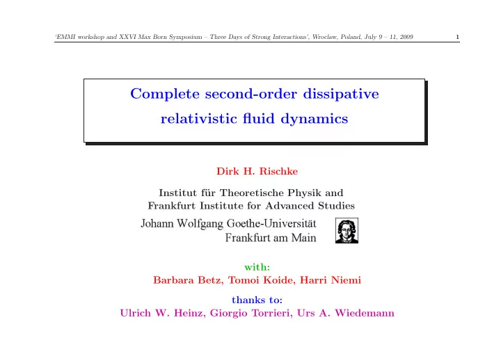
‘EMMI workshop and XXVI Max Born Symposium – Three Days of Strong Interactions’, Wroclaw, Poland, July 9 – 11, 2009 2 Preliminaries (I) Tensor decomposition of net charge current and energy-momentum tensor: N µ = n u µ + ν µ 1. Net charge current: u µ u µ = u µ g µν u ν = 1 u µ fluid 4-velocity, g µν ≡ diag(+ , − , − , − ) (West coast!!) metric tensor, n ≡ u µ N µ net charge density in fluid rest frame ν µ ≡ ∆ µν N ν diffusion current (flow of net charge relative to u µ ), ν µ u µ = 0 ∆ µν = g µν − u µ u ν projector onto 3-space orthogonal to u µ , ∆ µν u ν = 0 T µν = ǫ u µ u ν − ( p + Π) ∆ µν + 2 q ( µ u ν ) + π µν 2. Energy-momentum tensor: ǫ ≡ u µ T µν u ν energy density in fluid rest frame p pressure in fluid rest frame bulk viscous pressure, p + Π ≡ − 1 3 ∆ µν T µν Π q µ ≡ ∆ µν T νλ u λ heat flux current (flow of energy relative to u µ ), q µ u µ = 0 π µν ≡ T <µν> π µν u µ = π µν u ν = 0 , π µ shear stress tensor, µ = 0 a ( µν ) ≡ 1 2 ( a µν + a νµ ) symmetrized tensor a <µν> ≡ � � a αβ symmetrized, traceless spatial projection α ∆ ν ) β − 1 ∆ ( µ 3 ∆ µν ∆ αβ

‘EMMI workshop and XXVI Max Born Symposium – Three Days of Strong Interactions’, Wroclaw, Poland, July 9 – 11, 2009 3 Preliminaries (II) Fluid dynamical equations: 1. Net charge (e.g., strangeness) conservation: ∂ µ N µ = 0 ⇐ ⇒ ˙ n + n θ + ∂ · ν = 0 a ≡ u µ ∂ µ a ˙ convective (comoving) derivative (fluid rest frame, u µ RF ≡ g µ = ⇒ time derivative, ˙ a RF ≡ ∂ t a ) 0 θ ≡ ∂ µ u µ expansion scalar 2. Energy-momentum conservation: ∂ µ T µν = 0 ⇐ ⇒ energy conservation: u ν ∂ µ T µν = ˙ u − π µν ∂ µ u ν = 0 ǫ + ( ǫ + p + Π) θ + ∂ · q − q · ˙ acceleration equation: ∆ µν ∂ λ T νλ = 0 ⇐ ⇒ u µ = ∇ µ ( p +Π) − Π ˙ u µ − ∆ µν ˙ q ν − q µ θ − q ν ∂ ν u µ − ∆ µν ∂ λ π νλ ( ǫ + p ) ˙ ∇ µ ≡ ∆ µν ∂ ν 3-gradient (spatial gradient in fluid rest frame)

‘EMMI workshop and XXVI Max Born Symposium – Three Days of Strong Interactions’, Wroclaw, Poland, July 9 – 11, 2009 4 Preliminaries (III) Problem: 5 equations, but 15 unknowns (for given u µ ): ǫ , p , n , Π , ν µ (3) , q µ (3) , π µν (5) Solution: 1. clever choice of frame (Eckart, Landau,...): eliminate ν µ or q µ ⇒ does not help! Promotes u µ to dynamical variable! = 2. ideal fluid limit: all dissipative terms vanish, Π = ν µ = q µ = π µν = 0 ⇒ 6 unknowns: ǫ , p , n , u µ (3) = (not quite there yet...) = ⇒ fluid is in local thermodynamical equilibrium = ⇒ provide equation of state (EOS) p ( ǫ, n ) to close system of equations 3. provide additional equations for dissipative quantities = ⇒ dissipative relativistic fluid dynamics (a) First-order theories: e.g. generalization of Navier-Stokes (NS) equations to the relativistic case (Eckart, Landau-Lifshitz) (b) Second-order theories: e.g. Israel-Stewart (IS) equations

‘EMMI workshop and XXVI Max Born Symposium – Three Days of Strong Interactions’, Wroclaw, Poland, July 9 – 11, 2009 5 Preliminaries (IV) Navier-Stokes (NS) equations: Π NS = − ζ θ 1. bulk viscous pressure: ζ bulk viscosity NS = κ n q µ β ( ǫ + p ) ∇ µ α 2. heat flux current: β β ≡ 1 /T inverse temperature, α ≡ β µ , µ chemical potential, κ thermal conductivity π µν NS = 2 η σ µν 3. shear stress tensor: η shear viscosity, σ µν = ∇ <µ u ν> shear tensor = ⇒ algebraic expressions in terms of thermodynamic and fluid variables = ⇒ simple... but: unstable and acausal equations of motion!!

‘EMMI workshop and XXVI Max Born Symposium – Three Days of Strong Interactions’, Wroclaw, Poland, July 9 – 11, 2009 6 Motivation (I) 25 P. Romatschke, U. Romatschke, PRL 99 (2007) 172301 ideal Au+Au @ √ s = 200 AGeV η /s=0.03 20 η /s=0.08 η /s=0.16 charged particles, min. bias STAR v 2 (percent) 15 10 5 0 0 1 2 3 4 H. Song, U.W. Heinz, PRC 78 (2008) 024902 p T [GeV] (a) ideal hydro ideal hydro (b) ideal hydro (c) viscous hydro: simplified I-S eqn. viscous hydro: simplified I-S eqn. viscous hydro: simplified I-S eqn. viscous hydro: full I-S eqn. 0.2 η /s=0.08, τ π =3η /sT η /s=0.08, τ π =3η /sT η /s=0.08, τ π =3η /sT 3 3 3 e 0 =30 GeV/fm e 0 =30 GeV/fm e 0 =30 GeV/fm v 2 τ 0 =0.6fm/c τ 0 =0.6fm/c τ 0 =0.6fm/c 0.1 T dec =130 MeV T dec =130 MeV T dec =130 MeV Au+Au, b=7 fm Cu+Cu, b=7 fm Au+Au, b=7 fm SM-EOS Q SM-EOS Q EOS L 0 0 0.5 1 1.5 0 0.5 1 1.5 0 0.5 1 1.5 2 p T (GeV) p T (GeV) p T (GeV)

‘EMMI workshop and XXVI Max Born Symposium – Three Days of Strong Interactions’, Wroclaw, Poland, July 9 – 11, 2009 7 Motivation (II) Israel-Stewart (IS) equations: second-order, dissipative relativistic fluid dynamics W. Israel, J.M. Stewart, Ann. Phys. 118 (1979) 341 “Simplified” IS equations: e.g. shear stress tensor π <µν> + π µν = π µν τ π ˙ NS = ⇒ dynamical (instead of algebraic) equations for dissipative terms! π µν relaxes to its NS value π µν = ⇒ NS on the time scale τ π = ⇒ stable and causal fluid dynamical equations of motion! “Full” IS equations: NS − η  τ π   2 β π µν ∂ λ π <µν> + π µν = π µν η β u λ  + 2 τ π π <µ ω ν>λ τ π ˙   λ ω µν ≡ 1 2 ∆ µα ∆ νβ ( ∂ α u β − ∂ β u α ) vorticity

‘EMMI workshop and XXVI Max Born Symposium – Three Days of Strong Interactions’, Wroclaw, Poland, July 9 – 11, 2009 8 Motivation (III) = ⇒ Difference between “simplified” and “full” IS equations: the latter include higher-order terms? π µν π ν>λ 1 τ π ω µν ∼ δ ≪ 1 ⇒ τ π ω <µ ǫ ∼ δ 2 For instance, if ∼ δ ≪ 1 , = λ ǫ = ⇒ Goals: 1. What are the correct equations of motion for the dissipative quantities? = ⇒ develop consistent power counting scheme 2. Generalization to µ � = 0 (relevant for FAIR physics!) ⇒ include heat flux q µ = 3. Generalization to non-conformal fluids (relevant near T c !) = ⇒ include bulk viscous pressure Π

‘EMMI workshop and XXVI Max Born Symposium – Three Days of Strong Interactions’, Wroclaw, Poland, July 9 – 11, 2009 9 Results (I) Power counting: 3 length scales: 2 microscopic, 1 macroscopic • thermal wavelength λ th ∼ β ≡ 1 /T ℓ mfp ∼ ( � σ � n ) − 1 • mean free path n ∼ T 3 = β − 3 ∼ λ − 3 � σ � averaged cross section, th ∂ µ ∼ L − 1 • length scale over which macroscopic fluid fields vary L hydro , hydro λ 3 λ 3 ℓ mfp 1 1 ∼ η since η ∼ ( � σ � λ th ) − 1 = th th ∼ ∼ ∼ Note: ⇒ λ th � σ � n λ th � σ � λ th � σ � λ th s s ∼ n ∼ T 3 = β − 3 ∼ λ − 3 s entropy density, th η = ⇒ solely determined by the 2 microscopic length scales! s ζ κ Note: similar argument holds for s , β s

‘EMMI workshop and XXVI Max Born Symposium – Three Days of Strong Interactions’, Wroclaw, Poland, July 9 – 11, 2009 10 Results (II) 3 regimes: ℓ mfp ∼ η ⇒ � σ � ≪ λ 2 • dilute gas limit s ≫ 1 ⇐ th = ⇒ weak-coupling limit λ th ℓ mfp ∼ η ⇒ � σ � ∼ λ 2 • viscous fluids s ∼ 1 ⇐ th λ th interactions happen on the scale λ th = ⇒ moderate coupling ℓ mfp ∼ η ⇒ � σ � ≫ λ 2 • ideal fluid limit s ≪ 1 ⇐ th = ⇒ strong-coupling limit λ th ℓ mfp ℓ mfp ∂ µ ∼ ≡ K ∼ δ ≪ 1 gradient (derivative) expansion: L hydro K Knudsen number = ⇒ equivalent to k ℓ mfp ≪ 1 , k typical momentum scale R. Baier, P. Romatschke, D.T. Son, A.O. Starinets, M.A. Stephanov, JHEP 0804 (2008) 100 = ⇒ separation of macroscopic fluid dynamics (large scale ∼ L hydro ) from microscopic particle dynamics (small scale ∼ ℓ mfp )

‘EMMI workshop and XXVI Max Born Symposium – Three Days of Strong Interactions’, Wroclaw, Poland, July 9 – 11, 2009 11 Results (III) Dissipative quantities: Π , q µ , π µν Primary quantities: ǫ , p , n , s ⇐ ⇒ ǫ ∼ q µ ǫ ∼ π µν Π If K ∼ ℓ mfp ∂ µ ∼ δ ≪ 1 , then ∼ δ ≪ 1 ǫ Dissipative quantities are small compared to primary quantities = ⇒ small deviations from local thermodynamical equilibrium! ζ β s , η κ Note: statement independent of value of s , s ! Proof: Gibbs relation: ǫ + p = T s + µn = ⇒ β ǫ ∼ s ! Estimate dissipative terms by their Navier-Stokes values: NS = κ n π µν ∼ π µν q µ ∼ q µ β ( ǫ + p ) ∇ µ α , NS = 2 η σ µν Π ∼ Π NS = − ζ θ , β ⇒ Π ǫ ∼ − ζ β ǫ β θ ∼ − ζ β λ th ℓ mfp θ ∼ ℓ mfp ∂ µ u µ ∼ δ , = s λ th ℓ mfp q µ ǫ ∼ κ 1 β ( ǫ + p ) β ∇ µ α ∼ κ n β λ th ℓ mfp ∇ µ α ∼ ℓ mfp ∇ µ α ∼ δ , β β ǫ β s λ th ℓ mfp π µν ∼ 2 η β ǫ β σ µν ∼ 2 η β λ th ℓ mfp σ µν ∼ ℓ mfp ∇ <µ u ν> ∼ δ , q.e.d. ǫ s λ th ℓ mfp