Compact Data Strutures Antonio Faria, Javier D. Fernndez and Miguel - PowerPoint PPT Presentation
(To compress is to Conquer) Compact Data Strutures Antonio Faria, Javier D. Fernndez and Miguel A. Martinez-Prieto 3rd KEYSTONE Training School Keyword search in Big Linked Data 23 TH AUGUST 2017 Agenda Introduction Basic
(To compress is to Conquer) Compact Data Strutures Antonio Fariña, Javier D. Fernández and Miguel A. Martinez-Prieto 3rd KEYSTONE Training School Keyword search in Big Linked Data 23 TH AUGUST 2017
Agenda Introduction Basic compression Sequences Bit sequences Integer sequences A brief Review about Indexing PAGE 2 images: zurb.com
Introduction to Compact Data Structures “ Compact data structures lie at the intersection of Data Structures (indexing) and Information Theory (compression): One looks at data representations that not only permit space close to the minimum possible (as in compression) but also require that those representations allow one to efficiently carry out some operations on the data. PAGE 3 COMPACT DATA STRUCTURES: TO COMPRESS IS TO CONQUER
Introduction Why compression? 4 of 78 Disks are cheap !! But they are also slow ! Compression can help more data to fit in main memory. (access to memory is around 10 6 times faster than HDD) CPU speed is increasing faster We can trade processing time (needed to uncompress data) by space.
Introduction Why compression? 5 of 78 Compression does not only reduce space! I/O access on disks and networks Processing time * (less data has to be processed) … If appropriate methods are used For example: Allowing handling data compressed all the time. Doc 1 Doc 2 Doc 3 Doc n Compressed Text Doc 1 Doc 2 Doc 3 Doc n collection (30%) Text collection (100%) Doc 1 Doc 2 Doc 3 Doc n Let’s search for Compressed Text “Keystone" collection (20%) P7zip, others
Introduction Why indexing? 6 of 78 Indexing permits sublinear search time term 1 … Keystone … term n Index (> 5-30%) Doc 1 Doc 2 Doc 3 Doc n Doc 1 Doc 2 Doc 3 Doc n Compressed Text collection (30%) Text collection (100%) Let’s search for “Keystone"
Introduction Why compact data structures? 7 of 78 Self-indexes: sublinear search time term 1 Text implicitly kept … Keystone … term n Index (> 5-30%) Doc 1 Doc 2 Doc 3 Doc n Self-index (WT , WCSA,…) Text collection term 1 1 0 0 0 1 1 0 … Let’s search for 0 1 Keystone “Keystone" … 0 1 0 0 0 1 0 term n
Agenda Introduction Basic compression Sequences Bit sequences Integer sequences A brief Review about Indexing PAGE 8 images: zurb.com
Compression “ Compressing aims at representing data within less space. How does it work? Which are the most traditional compression techniques? PAGE 9 COMPACT DATA STRUCTURES: TO COMPRESS IS TO CONQUER
Basic Compression Modeling & Coding 10 of 78 A compressor could use as a source alphabet: A fixed number of symbols (statistical compressors) 1 char, 1 word A variable number of symbols (dictionary-based compressors) 1st occ of ‘ a ’ encoded alone, 2nd occ encoded with next one ‘ a x ’ Codes are built using symbols of a target alphabet: Fixed length codes (10 bits, 1 byte, 2 bytes, …) Variable length codes (1,2,3,4 bits/bytes …) Classification ( fixed-to-variable, variable-to-fixed ,…) Target alphabet fixed var statistical -- fixed Input alphabet var dictionary var2var
Basic Compression Main families of compressors 11 of 78 Taxonomy Dictionary based (gzip, compress , p7zip… ) Grammar based (BPE, Repair) Statistical compressors (Huffman, arithmetic , Dense, PPM,… ) Statistical compressors Gather the frequencies of the source symbols. Assign shorter codewords to the most frequent symbols. Obtain compression
Basic Compression Dictionary-based compressors 12 of 78 How do they achieve compression? Assign fixed-length codewords to variable-length symbols (text substrings) The longer the replaced substring the better compression Well-known representatives: Lempel-Ziv family LZ77 (1977): GZIP, PKZIP, ARJ, P7zip LZ78 (1978) LZW (1984): Compress, GIF images
Basic Compression LZW 13 of 78 EXAMPLE Starts with an initial dictionary D (contains symbols in S ) For a given position of the text. while D contains w, reads prefix w=w 0 w 1 w 2 … If w 0 …w k w k+1 is not in D (w 0 …w k does!) output (i = entryPos(w 0 …w k )) (Note: codeword = log 2 (|D|)) Add w 0 …w k w k+1 to D Continue from w k+1 on (included) Dictionary has limited length? Policies: LRU, truncate& go, …
Basic Compression LZW 14 of 78 EXAMPLE Starts with an initial dictionary D (contains symbols in S ) For a given position of the text. while D contains w, reads prefix w=w 0 w 1 w 2 … If w 0 …w k w k+1 is not in D (w 0 …w k does!) output (i = entryPos(w 0 …w k )) (Note: codeword = log 2 (|D|)) Add w 0 …w k w k+1 to D Continue from w k+1 on (included) Dictionary has limited length? Policies: LRU, truncate& go, …
Basic Compression Grammar-based – BPE - Repair 15 of 78 Replaces pairs of symbols by a new one, until no pair repeats twice Adds a rule to a Dictionary. DE G A B C D E A B D E F D E D E F A B E C D Source sequence A B C G A B G F G G F A B E C D AB H H C G H G F G G F H E C D GF I Dictionary of Rules Final Repair Sequence H C G H I G I H E C D
Basic Compression Statistical compressors 16 of 78 Assign shorter codewords to the most frequent symbols Must gather symbol frequencies for each symbol c in S . Compression is lower bounded by the (zero-order) empirical entropy of the sequence (S). n= num of symbols n c = occs of symbol c H 0 (S) <= log (| S |) n H 0 (S) = lower bound of the size of S compressed with a zero-order compressor Most representative method: Huffman coding
Basic Compression Statistical compressors: Huffman coding 17 of 78 Optimal prefix free coding No codeword is a prefix of one another. Decoding requires no look-ahead! Asymptotically optimal: |Huffman(S)| <= n(H0(S)+1) Typically using bit-wise codewords Yet D-ary Huffman variants exist (D=256 byte-wise) Builds a Huffman tree to generate codewords
Basic Compression Statistical compressors: Huffman coding 18 of 78 Sort symbols by frequency: S= ADBAAAABBBBCCCCDDEEE
Basic Compression Statistical compressors: Huffman coding 19 of 78 Bottom – Up tree construction
Basic Compression Statistical compressors: Huffman coding 20 of 78 Bottom – Up tree construction
Basic Compression Statistical compressors: Huffman coding 21 of 78 Bottom – Up tree construction
Basic Compression Statistical compressors: Huffman coding 22 of 78 Bottom – Up tree construction
Basic Compression Statistical compressors: Huffman coding 23 of 78 Bottom – Up tree construction
Basic Compression Statistical compressors: Huffman coding 24 of 78 Branch labeling
Basic Compression Statistical compressors: Huffman coding 25 of 78 Code assignment
Basic Compression Statistical compressors: Huffman coding 26 of 78 Compression of sequence S= ADB… ADB… 01 000 10 …
Basic Compression Burrows-Wheeler Transform (BWT) 27 of 78 Given S= mississipii$, BWT(S) is obtained by: (1) creating a Matrix M with all circular permutations of S$, (2) sorting the rows of M, and (3) taking the last column. mississippi$ $mississippi $mississippi i$mississipp i$mississipp ippi$mississ pi$mississip issippi$miss ppi$mississi ississippi$m sort ippi$mississ mississippi$ sippi$missis pi$mississip ssippi$missi ppi$mississi issippi$miss sippi$missis sissippi$mis sissippi$mis ssissippi$mi ssippi$missi ississippi$m ssissippi$mi L = BWT(S) F
Basic Compression Burrows-Wheeler Transform: reversible (BWT -1 ) 28 of 78 Given L=BWT(S), we can recover S=BWT -1 (L) Steps: 1. Sort L to obtain F 1 $mississippi 2 2. Build LF mapping so that 2 i$mississipp 7 If L[i]=‘c’ , and 3 ippi$mississ 9 k = the number of times ‘c’ occurs in L [1..i], and j= position in F of the k th occurrence of ‘c’ 10 4 issippi$miss Then set LF[i]=j 5 ississippi$m 6 6 mississippi$ 1 Example : L[7] = ‘p’, it is the 2nd ‘p’ in L LF[7] = 8 7 pi$mississip 8 which is the 2nd occ of ‘p’ in F 8 ppi$mississi 3 9 sippi$missis 11 12 10 sissippi$mis 11 ssippi$missi 4 12 ssissippi$mi 5 L LF F
Basic Compression Burrows-Wheeler Transform: reversible (BWT -1 ) 29 of 78 Given L=BWT(S), we can recover S=BWT -1 (L) Steps: 1. Sort L to obtain F 1 $mississippi 2 - 2. Build LF mapping so that 2 i$mississipp 7 - If L[i]=‘c’ , and 3 ippi$mississ 9 k = the number of times ‘c’ occurs in L [1..i], and - j= position in F of the k th occurrence of ‘c’ 10 4 issippi$miss - Then set LF[i]=j 5 ississippi$m 6 - 6 mississippi$ 1 - Example : L[7] = ‘p’, it is the 2nd ‘p’ in L LF[7] = 8 7 pi$mississip 8 - which is the 2nd occ of ‘p’ in F 8 ppi$mississi 3 - 3. Recover the source sequence S in n steps: 9 sippi$missis 11 - Initially p=l=6 (position of $ in L); i=0; n=12; 12 10 sissippi$mis - In each step: S[n-i] = L[p]; 11 ssippi$missi 4 - p = LF[p]; 12 ssissippi$mi 5 $ i = i+1; L LF S F
Recommend
More recommend
Explore More Topics
Stay informed with curated content and fresh updates.
