Coefficient of Correlation The regression equation Y = 0 + 1 x + - PowerPoint PPT Presentation

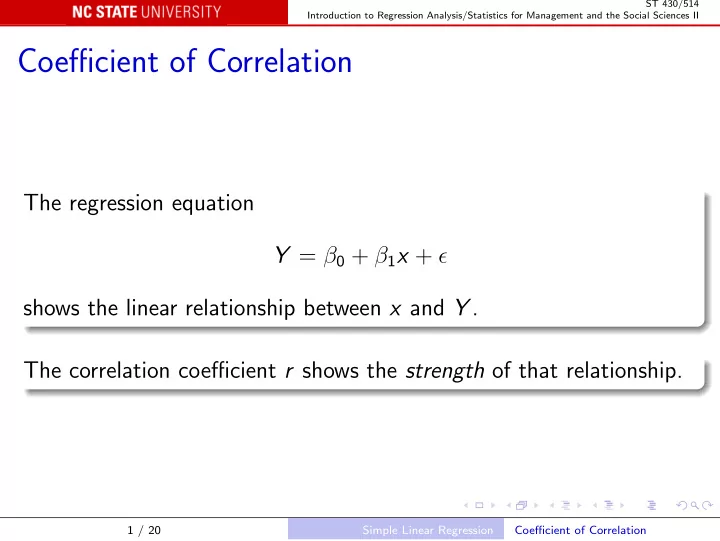
ST 430/514 Introduction to Regression Analysis/Statistics for Management and the Social Sciences II Coefficient of Correlation The regression equation Y = β 0 + β 1 x + ǫ shows the linear relationship between x and Y . The correlation coefficient r shows the strength of that relationship. 1 / 20 Simple Linear Regression Coefficient of Correlation

ST 430/514 Introduction to Regression Analysis/Statistics for Management and the Social Sciences II Properties of r r always lies between -1 and +1; r = 1 when x and y have a perfect positive linear relationship; r = − 1 when x and y have a perfect negative linear relationship; r = 0 when there is no relationship. 2 / 20 Simple Linear Regression Coefficient of Correlation

ST 430/514 Introduction to Regression Analysis/Statistics for Management and the Social Sciences II Calculate r directly as � x i y i − n ¯ � ( x i − ¯ x )( y i − ¯ y ) x ¯ y r = y ) 2 = . ( � x 2 x 2 ) ( � y 2 �� ( x i − ¯ � x ) 2 � ( y i − ¯ y 2 ) i − n ¯ i − n ¯ Calculate r from ˆ β 1 as �� ( x i − ¯ x ) 2 β 1 × s x r = ˆ y ) 2 = ˆ β 1 × . � ( y i − ¯ s y Note that r always has the same sign as ˆ β 1 . 3 / 20 Simple Linear Regression Coefficient of Correlation

ST 430/514 Introduction to Regression Analysis/Statistics for Management and the Social Sciences II Correlation and Causation Not the same thing! A 1999 article in the journal Nature found “a strong association between myopia and night-time ambient light exposure during sleep in children before they reach two years of age”. The article noted that no causal link was established, but continued “it seems prudent that infants and young children sleep at night without artificial lighting in the bedroom”. Much anguish for parents of myopic children! 4 / 20 Simple Linear Regression Coefficient of Correlation

ST 430/514 Introduction to Regression Analysis/Statistics for Management and the Social Sciences II Later studies found that myopic parents tend to leave the light on, and also tend to have myopic children. One study, in particular, found that “the proportion of myopic children in those subjected to a range of nursery-lighting conditions is remarkably uniform”. This suggests that the association observed in the first study resulted from parental behavior and inheritance, not from a causal effect of night-time lighting. The moral: “Correlation does not imply causation”. 5 / 20 Simple Linear Regression Coefficient of Correlation

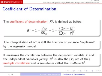
ST 430/514 Introduction to Regression Analysis/Statistics for Management and the Social Sciences II Coefficient of Determination The coefficient of determination R 2 also measures the strength of the relationship between x and y . With only one independent variable, R 2 = r 2 . When we have more than one independent variable, R 2 measures the strength of the relationship of y to all of them. The correlation coefficient r is always between pairs of individual variables. 6 / 20 Simple Linear Regression Coefficient of Determination

ST 430/514 Introduction to Regression Analysis/Statistics for Management and the Social Sciences II We interpret R 2 as the fraction of the variance of y that is “explained” by the regression. The definition is � ( y i − ˆ y i ) 2 R 2 = 1 − SS E = 1 − y ) 2 . SS yy � ( y i − ¯ If the regression is strong, we expect ˆ y i to be a good predictor of y i , so SS E << SS yy , whence the ratio is small and R 2 is close to 1. Conversely, if the regression is weak, ˆ y i is not much better than ¯ y as a predictor of y i , so the ratio is close to 1 and R 2 is close to 0. 7 / 20 Simple Linear Regression Coefficient of Determination

ST 430/514 Introduction to Regression Analysis/Statistics for Management and the Social Sciences II Estimation and Prediction An attractive feature of a regression equation like E ( Y | x ) = β 0 + β 1 x is that it is valid for values of x other than those in the data set, x 1 , x 2 , . . . , x n . That is, we can use it to estimate what E ( Y | x ) would be for some x that was not part of the experiment. But ...using it for some x that is far from all of x 1 , x 2 , . . . , x n is extrapolation, and runs the risk that the model may not be a good approximation. 8 / 20 Simple Linear Regression Estimation and Prediction

ST 430/514 Introduction to Regression Analysis/Statistics for Management and the Social Sciences II Estimation The estimate of E ( Y | x = x p ) for some particular x p is y ( x p ) = ˆ β 0 + ˆ ˆ β 1 x p . This is a statistic , so it has a sampling distribution : it is unbiased: y ( x p )] = E (ˆ β 0 + ˆ E [ˆ β 1 x p ) = β 0 + β 1 x p = E ( Y | x = x p ); its standard error is � n + ( x p − ¯ 1 x ) 2 y ( x p ) = σ σ ˆ . SS xx 9 / 20 Simple Linear Regression Estimation and Prediction

ST 430/514 Introduction to Regression Analysis/Statistics for Management and the Social Sciences II Example: in the advertising/sales case, the least squares line is y ( x ) = − 0 . 1 + 0 . 7 x . ˆ So if x = 4 (advertising expenditure = $400), we estimate the expected revenue to be y (4) = 2 . 7 , ˆ or $2,700. The estimated standard error of this estimate is � 5 + (4 − 3) 2 1 0 . 61 × = 0 . 332 . 10 or $332. 10 / 20 Simple Linear Regression Estimation and Prediction

ST 430/514 Introduction to Regression Analysis/Statistics for Management and the Social Sciences II Prediction Note: y ( x p ) = ˆ β 0 + ˆ ˆ β 1 x p is the estimate of E ( Y | x = x p ), the expected value of Y when x = x p . Sometimes we want to predict the actual value of Y for a new observation at x = x p . Example: if the store spends $400 on advertising next month , what can we predict about revenue? 11 / 20 Simple Linear Regression Estimation and Prediction

ST 430/514 Introduction to Regression Analysis/Statistics for Management and the Social Sciences II Our best guess, the predicted value, is still ˆ y ( x p ). But the error is larger: the standard error of prediction is � x ) 2 1 + 1 n + ( x p − ¯ σ [ y − ˆ y ( x p )] = σ . SS xx Compare with � n + ( x p − ¯ 1 x ) 2 σ ˆ y ( x p ) = σ . SS xx In the example, ˆ σ [ y − ˆ y (4)] = 0 . 690, or $690. 12 / 20 Simple Linear Regression Estimation and Prediction

ST 430/514 Introduction to Regression Analysis/Statistics for Management and the Social Sciences II More generally, we might want to predict the average of m > 1 new observations at x = x p . Our best guess, the predicted value, is again ˆ y ( x p ). The standard error is between σ ˆ y ( x p ) and σ [ y − ˆ y ( x p )] : � m + 1 1 n + ( x p − ¯ x ) 2 σ . SS xx The predicted value and standard error are the same if the new observations are made at different x s whose mean is x p . 13 / 20 Simple Linear Regression Estimation and Prediction

ST 430/514 Introduction to Regression Analysis/Statistics for Management and the Social Sciences II Fire Damage How does the cost of fire damage vary with distance from the nearest fire station? Here x is distance in miles, and y is the cost of damage. Steps in the analysis (not quite the same as in the text): Plot the data: 1 firedam <- read.table("Text/Exercises&Examples/FIREDAM.txt", header = TRUE) plot(firedam) The plot shows approximately linear dependence. 14 / 20 Simple Linear Regression Complete Example

ST 430/514 Introduction to Regression Analysis/Statistics for Management and the Social Sciences II Overlay the least squares line: 2 firedam.lm <- lm(DAMAGE ~ DISTANCE, data = firedam) abline(reg = firedam.lm, col = "blue") No obvious issues. 15 / 20 Simple Linear Regression Complete Example

ST 430/514 Introduction to Regression Analysis/Statistics for Management and the Social Sciences II Summarize the fitted model: 3 summary(firedam.lm) Least squares line: ˆ y = 10 . 2779 + 4 . 9193 x . Residual standard error: 2.316 on 13 degrees of freedom Test H 0 : β 1 = 0: t = 12 . 525 with the same 13 degrees of freedom; Pr( > | t | ) = 1 . 25 × 10 − 8 ; very strong evidence against H 0 . 95% Confidence Interval: 4 . 071 < β 1 < 5 . 768; Coefficient of Determination: 0.9235. 16 / 20 Simple Linear Regression Complete Example

ST 430/514 Introduction to Regression Analysis/Statistics for Management and the Social Sciences II Using multiple regression (next topic), check whether the 4 straight line model is adequate by fitting the quadratic model E ( Y ) = β 0 + β 1 x + β 2 x 2 and testing H 0 : β 2 = 0. Use graphical regression diagnostics (later topic) to check the 5 residuals for issues. 17 / 20 Simple Linear Regression Complete Example

ST 430/514 Introduction to Regression Analysis/Statistics for Management and the Social Sciences II Regression Through the Origin In the usual straight-line model E ( Y ) = β 0 + β 1 x , the intercept β 0 is estimated from the data. In some situations we may know that E ( Y ) = 0 when x = 0, or in other words that β 0 = 0. We should then fit the simpler “regression through the origin” model E ( Y ) = β 1 x . 18 / 20 Simple Linear Regression Regression Through the Origin