Cluster Analysis Applied Multivariate Statistics Spring 2012 - PowerPoint PPT Presentation
Cluster Analysis Applied Multivariate Statistics Spring 2012 Overview Hierarchical Clustering: Agglomerative Clustering Partitioning Methods: K-Means and PAM Gaussian Mixture Models 1 Goal of clustering Find groups, so that
Cluster Analysis Applied Multivariate Statistics – Spring 2012
Overview Hierarchical Clustering: Agglomerative Clustering Partitioning Methods: K-Means and PAM Gaussian Mixture Models 1
Goal of clustering Find groups, so that elements within cluster are very similar and elements between cluster are very different Problem: Need to interpret meaning of a group Examples: - Find customer groups to adjust advertisement - Find subtypes of diseases to fine-tune treatment Unsupervised technique: No class labels necessary N samples, k cluster: k N possible assignments E.g. N=100, k=5: 5 100 = 7*10 69 !! Thus, impossible to search through all assignments 2
Clustering is useful in 3+ dimensions Human eye is extremely good at clustering Use clustering only, if you can not look at the data (i.e. more than 2 dimensions) 3
Hierarchical Clustering Agglomerative: Build up cluster from individual observations Divisive: Start with whole group of observations and split off clusters Divisive clustering has much larger computational burden We will focus on agglomerative clustering Solve clustering for all possible numbers of cluster (1, 2, …, N) at once Choose desired number of cluster later 4
Agglomerative Clustering Data in 2 dimensions Clustering tree = Dendrogramm dissimilarity abcde b a cde c e de d ab 0 a b c d e Join samples/cluster that are closest until only one cluster is left 5
Agglomerative Clustering: Cutting the tree Clustering tree = Dendrogramm Get cluster solutions by cutting dissimilarity the tree: abcde - 1 Cluster: abcde (trivial) - 2 Cluster: ab - cde - 3 Cluster: ab – c – de cde - 4 Cluster: ab – c – d – e - 5 Cluster: a – b – c – d – e de ab 0 a b c d e 6
Dissimilarity between samples Any dissimilarity we have seen before can be used - euclidean - manhattan - simple matching coefficent - Jaccard dissimilarity - Gower’s dissimilarity - etc. 7
Dissimilarity between cluster Based on dissimilarity between samples Most common methods: - single linkage - complete linkage - average linkage No right or wrong: All methods show one aspect of reality If in doubt, I use complete linkage 8
Single linkage Distance between two cluster = minimal distance of all element pairs of both cluster Suitable for finding elongated cluster 9
Complete linkage Distance between two cluster = maximal distance of all element pairs of both cluster Suitable for finding compact but not well separated cluster 10
Average linkage Distance between two cluster = average distance of all element pairs of both cluster Suitable for finding well separated, potato-shaped cluster 11
Choosing the number of cluster No strict rule Find the largest vertical “drop” in the tree 12
Quality of clustering: Silhouette plot One value S(i) in [0,1] for each observation Compute for each observation i: a(i) = average dissimilarity between i and all other points of the cluster to which i belongs b(i) = average dissimilarity between i and its “neighbor” cluster, i.e., the nearest one to which it does not belong. (𝑐 𝑗 −𝑏 𝑗 ) Then, S(i) = (𝑏 𝑗 ,𝑐 𝑗 ) max S(i) large: well clustered; S(i) small: badly clustered S(i) negative: assigned to wrong cluster 1 1 Average S over 0.5 is acceptable S(1) small S(1) large 13
Silhouette plot: Example 14
Agglomerative Clustering in R Pottery Example Functions “ hclust ”, “ cutree ” in package “stats” Alternative: Function “ agnes ” in package “cluster” Function “silhouette” in package “cluster” 15
Partitioning Methods: K-Means Number of clusters K is fixed in advance Find K cluster centers 𝜈 𝑗 and assignments, so that within-groups Sum of Squares (WGSS) is minimal 𝑦 𝑗 − 𝜈 𝑗 2 𝑋𝐻𝑇𝑇 = 𝑏𝑚𝑚𝐷𝑚𝑣𝑡𝑢𝑓𝑠𝐷 𝑄𝑝𝑗𝑜𝑢𝑗𝑗𝑜𝐷𝑚𝑣𝑡𝑢𝑓𝑠𝐷 x x x x WGSS small WGSS large 16
K-Means Exact solution computationally infeasible Approximate solutions, e.g. Lloyd’s algorithm Different starting assignments will give different solutions Random restarts to avoid local optima Iterate until convergence 17
K-Means: Number of clusters • Run k-Means for several number of groups • Plot WGSS vs. number of groups • Choose number of groups after the last big drop of 18
Robust alternative: PAM Partinioning around Medoids (PAM) K-Means: Cluster center can be an arbitrary point in space PAM: Cluster center must be an observation (“ medoid ”) Advantages over K-means: - more robust against outliers - can deal with any dissimilarity measure - easy to find representative objects per cluster (e.g. for easy interpretation) 19
Partitioning Methods in R Function “ kmeans ” in package “stats” Function “pam” in package “cluster” Pottery revisited 20
Gaussian Mixture Models (GMM) Up to now: Heuristics using distances to find cluster Now: Assume underlying statistical model Gaussian Mixture Model: 𝐿 𝑔 𝑦; 𝑞, 𝜄 = 𝑞 𝑘 𝑘 𝑦; 𝜄 𝑘 𝑘=1 K populations with different probability distributions Example: X 1 ~ N(0,1), X 2 ~ N(2,1); p 1 = 0.2, p 2 = 0.8 1 1 2 ¼ exp( ¡ x 2 = 2) + 0 : 8 ¢ 2 ¼ exp( ¡ ( x ¡ 2) 2 = 2) f ( x ; p; µ ) = 0 : 2 ¢ p p Find number of classes and parameters 𝑞 𝑘 and 𝜄 𝑘 given data Assign observation x to cluster j, where estimated value of 𝑄 𝑑𝑚𝑣𝑡𝑢𝑓𝑠𝑘 𝑦 =𝑞 𝑘 𝑘 (𝑦; 𝜄 𝑘 ) 𝑔(𝑦; 𝑞, 𝜄) is largest 21
Revision: Multivariate Normal Distribution ¡ ¢ 1 ¡ 1 2 ¢ ( x ¡ ¹ ) T § ¡ 1 ( x ¡ ¹ ) p f ( x ; ¹; §) = 2 ¼ j § j exp 22
GMM: Example estimated manually • 3 clusters • p 1 = 0.7, p 2 = 0.2, p 3 = 0.1 • Mean vector and cov. Matrix per cluster p 1 = 0.7 x p 2 = 0.2 x p 3 = 0.1 x 23
Fitting GMMs 1/2 Maximum Likelihood Method Hard optimization problem Simplification: Restrict Covariance matrices to certain patterns (e.g. diagonal) 24
Fitting GMMs 2/2 Problem: Fit will never get worse if you use more cluster or allow more complex covariance matrices → How to choose optimal model ? Solution: Trade-off between model fit and model complexity BIC = log-likelihood – log(n)/2*(number of parameters) Find solution with maximal BIC 25
GMMs in R Function “ Mclust ” in package “ mclust ” Pottery revisited 26
Giving meaning to clusters Generally hard in many dimensions Look at position of cluster centers or cluster representatives (esp. easy in PAM) 27
(Very) small runtime study Uniformly distributed points in [0,1] 5 on my desktop 1 Mio samples with k-means: 5 sec (always just one replicate; just to give you a rough idea…) Good for small / medium data sets Good for huge data sets 28
Comparing methods Partitioning Methods: + Super fast (“millions of samples”) - No underlying Model Agglomerative Methods: + Get solutions for all possible numbers of cluster at once - slow (“thousands of samples”) GMMs: + Get statistical model for data generating process + Statistically justified selection of number of clusters - very slow (“hundreds of samples”) 29
Concepts to know Agglomerative clustering, dendrogram, cutting a dendrogram, dissimilarity measures between cluster Partitioning methods: k-Means, PAM GMM Choosing number of clusters: - drop in dendrogram - drop in WGSS - BIC Quality of clustering: Silhouette plot 30
R functions to know Functions “ kmeans ”, “ hclust ”, “ cutree ” in package “stats” Functions “pam”, “ agnes ”, “ shilouette ” in package “cluster” Function “ Mclust ” in package “ mclust ” 31
Recommend
More recommend
Explore More Topics
Stay informed with curated content and fresh updates.
