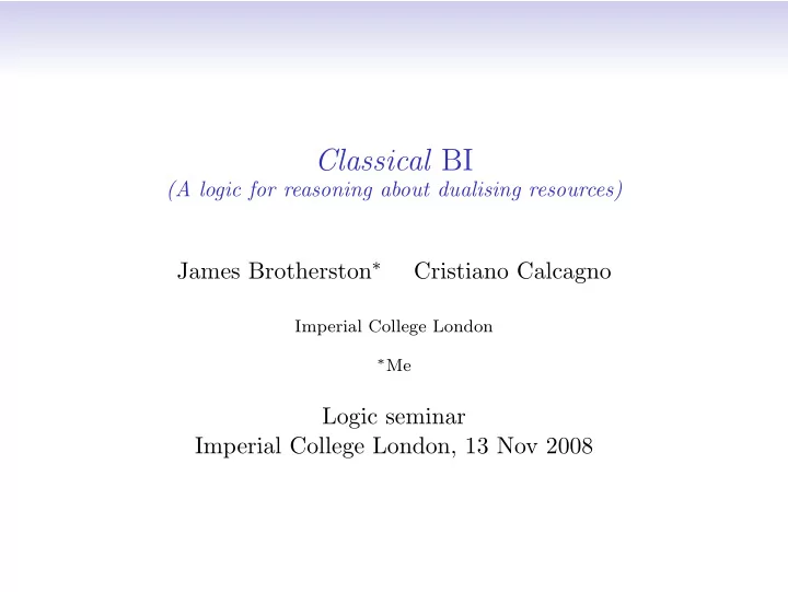
Classical BI (A logic for reasoning about dualising resources) James - PowerPoint PPT Presentation

Classical BI (A logic for reasoning about dualising resources) James Brotherston ∗ Cristiano Calcagno Imperial College London ∗ Me Logic seminar Imperial College London, 13 Nov 2008

BI : the logic of bunched implications (O’Hearn and Pym ’99) • A substructural logic with natural resource interpretation. • BI formula connectives: Additive: ⊤ ⊥ ¬ ∧ ∨ → Multiplicative: ⊤ ∗ ∗ — ∗ • Two flavours: • BI ( intuitionistic additives) • Boolean BI ( classical additives) • Our main reference point: Boolean BI (BBI). • Killer application of BBI: separation logic.

Our contribution: classical BI ( CBI ) • Why aren’t there multiplicative versions of ⊥ , ¬ , ∨ ? • We obtain CBI by adding them to BBI: Additive: ⊤ ⊥ ¬ ∧ ∨ → ∗ Multiplicative: ⊤ ∗ ⊥ ∗ ∼ ∗ ∨ — ∗ and considering both families to behave classically. • Are there non-trivial models of CBI? • How do we interpret the new connectives? • Is there a nice proof theory?

Part I Model theory

Algebraic semantics of BBI • Models of BBI are partial commutative monoids � R, ◦ , e � . • � R, ◦ , e � is understood as an abstract model of resource: R: a set of resources ◦ : a way of (partially) combining resources e: the distinguished empty resource • E.g., separation logic model � H, ♯, emp � , where: H: the set of heaps = def V ar ⇀ fin V al ♯ : domain-disjoint union of heaps emp: the empty heap s.t. emp( x ) undefined all x ∈ V ar

Interpreting the BBI connectives • An environment for M = � R, ◦ , e � is a map ρ : V → R . • We have the satisfaction relation r | = F : r | = P ⇔ r ∈ ρ ( P ) . . . r | = F 1 ∧ F 2 ⇔ r | = F 1 and r | = F 2 . . . r | = ⊤ ∗ ⇔ r = e r | = F 1 ∗ F 2 ⇔ r = r 1 ◦ r 2 and r 1 | = F 1 and r 2 | = F 2 ∀ r ′ . r ◦ r ′ defined and r ′ | = F 1 implies r ◦ r ′ | r | = F 1 — ∗ F 2 ⇔ = F 2 • A formula F is BBI-valid iff, in every BBI-model M , we have r | = F for all r ∈ R and all environments for M .

Dualising resource models of CBI • A CBI-model is given by a tuple � R, ◦ , e, − , ∞� , where: • � R, ◦ , e � is a partial commutative monoid; • ∞ ∈ R and − : R → R ; • for all r ∈ R , − r is the unique solution to r ◦ − r = ∞ . • Natural interpretation: models of dualising resources. • Clearly CBI-models are (special) BBI-models. • Every Abelian group is a CBI-model (with ∞ = e ).

Interpreting the CBI connectives ∗ ≡ ∼ F . • Main problem: we want ∼∼ F ≡ F but also F — ∗ ⊥ • Temporarily define atomic formula ⊲ ⊳ by: r | ⊳ ⇔ r = ∞ = ⊲ • Key observation: − r | = F ⇔ r | = ¬ ( F — ∗ ¬ ⊲ ⊳ ) ∗ , ∼ , ∗ • Thus we interpret ⊥ ∨ as follows: ∗ r | = ⊥ ⇔ r � = ∞ r | = ∼ F ⇔ − r �| = F = F 1 ∗ r | ∨ F 2 ⇔ ∀ r 1 , r 2 . − r ∈ r 1 ◦ r 2 implies − r 1 | = F 1 or − r 2 | = F 2 • CBI-validity is as for BBI.

Some semantic equivalences of CBI ∼⊤ ≡ ⊥ ∼⊤ ∗ ≡ ⊥ ∗ ∼∼ F ≡ F F — ∗ ⊥ ∗ ≡ ∼ F ¬∼ F ≡ ∼¬ F F ∗ ∨ G ≡ ∼ ( ∼ F ∗ ∼ G ) ∼ F ∗ F — ∗ G ≡ ∨ G F — ∗ G ≡ ∼ G — ∗ ∼ F F ∗ ∨ ⊥ ∗ ≡ F

Example: Personal finance • Let � Z , + , 0 , −� be the Abelian group of integers. • View m ∈ Z as money ( £ ): • m > 0: credit • m < 0: debt • m | = F means “ £ m is enough to make F true”. • Let C be the formula “I’ve enough money to buy cigarettes (£ 5 )” and W be “I’ve enough to buy whisky (£ 20 )” . So: m | = C ⇔ m ≥ 5 m | = W ⇔ m ≥ 20

Example contd.: Personal finance • m | = C ∧ W ⇔ m | = C and m | = W ⇔ m ≥ 20 “I have enough to buy cigarettes and also to buy whisky” • m | = C ∗ W ⇔ m = m 1 + m 2 and m 1 | = C and m 2 | = W ⇔ m ≥ 25 “I have enough to buy both cigarettes and whisky” ∀ m ′ . m ′ | = C implies m + m ′ | • m | ∗ W ⇔ = C — = W ⇔ m ≥ 15 “if I acquire enough money to buy cigarettes then, in total, I have enough to buy whisky”

Example contd.: Personal finance • m | = ⊥ ∗ ⇔ m � = 0 “I am either in credit or in debt” • m | = ∼ C ⇔ − m �| = C ⇔ m > − 5 “I owe less than the price of a pack of cigarettes” = C ∗ • m | ∨ W ⇔ ∀ m 1 , m 2 . − m = m 1 + m 2 implies − m 1 | = C or − m 2 | = W ⇔ m ≥ 24 Note that C ∗ ∨ W ⇔ ∼ C — ∗ W ⇔ ∼ W — ∗ C , i.e.: “if I spend less than the price of a pack of cigarettes, then I will still have enough money to buy whisky (and vice versa!)”

Part II Proof theory

Bunches • Bunches Γ are given by: Γ ::= F | ∅ | ∅ | Γ; Γ | Γ , Γ • Bunches represent formulas at the meta-level: Antecedent meaning ∅ ⊤ ⊤ ∗ ∅ ; ∧ ∗ , • ‘;’ and ‘,’ associative and commutative with units ∅ resp. ∅ . • Weakening and contraction hold for ‘;’ but not ‘,’. • Γ(∆) is notation for: ∆ is a sub-bunch occurring in Γ.

Sequent calculus rules for (B)BI Γ( F 1 ; F 2 ) ⊢ F Γ ⊢ F Γ ⊢ G ( ∧ L) ( ∧ R) Γ( F 1 ∧ F 2 ) ⊢ F Γ ⊢ F ∧ G Γ( F 1 , F 2 ) ⊢ F Γ ⊢ F 1 ∆ ⊢ F 2 ( ∗ R) ( ∗ L) Γ( F 1 ∗ F 2 ) ⊢ F Γ , ∆ ⊢ F 1 ∗ F 2 ∆ ⊢ F 1 Γ(∆; F 2 ) ⊢ F Γ; F 1 ⊢ F 2 ( → L) ( → R) Γ(∆; F 1 → F 2 ) ⊢ F Γ ⊢ F 1 → F 2 • Cut-elimination holds for BI sequent calculus (Pym 2002). • For BBI, need to add a rule like: Γ ⊢ ¬¬ F (RAA) Γ ⊢ F

Sequent calculus for CBI • Obvious approach for CBI: write two-sided sequents Γ ⊢ ∆ where Γ , ∆ are bunches. • Natural rules for the negations: Γ ⊢ F ; ∆ Γ; F ⊢ ∆ ( ¬ L) ( ¬ R) Γ; ¬ F ⊢ ∆ Γ ⊢ ¬ F ; ∆ Γ ⊢ F, ∆ Γ , F ⊢ ∆ ( ∼ L) ( ∼ R) Γ , ∼ F ⊢ ∆ Γ ⊢ ∼ F, ∆ • But there are no cut-free proofs of e.g. A, ( B ; ¬ B ) ⊢ C ∼¬ F ⊢ ¬∼ F • Alternative formulation of rules for negation?

DL CBI : a display calculus proof system for CBI • We give a display calculus ´ a la Belnap for CBI. • Write consecutions X ⊢ Y , where X, Y are structures: X ::= F | ∅ | ∅ | ♯X | ♭X | X ; X | X, X • Here the negations are represented at the meta-level: Antecedent meaning Consequent meaning ∅ ⊤ ⊥ ⊤ ∗ ⊥ ∗ ∅ ¬ ¬ ♯ ♭ ∼ ∼ ∧ ∨ ; ∗ , ∗ ∨

Proof rules for DL CBI Three types of proof rules: 1. display postulates allowing structures to be shuffled: X ; Y ⊢ Z X ⊢ Y = = = = = = = = = = = = = = X ⊢ ♯Y ; Z ♯Y ⊢ ♯X 2. left- and right-introduction rules for each logical connective: X ⊢ F G ⊢ Y X, F ⊢ G (— ∗ L) (— ∗ R) ∗ G ⊢ ♭X, Y F — X ⊢ F — ∗ G 3. structural rules governing the structural connectives: W ; ( X ; Y ) ⊢ Z X ⊢ Z X ⊢ Y, ∅ = = = = = = = = = = = (AAL) (WkR) = = = = = = = (MIR) ( W ; X ); Y ⊢ Z X ⊢ Y ; Z X ⊢ Y

Results about DL CBI Easy consequence of the fact that DL CBI is a display calculus: Theorem (Cut-elimination) Any DL CBI proof of X ⊢ Y can be transformed into a cut-free proof of X ⊢ Y . Main technical results: (NB. Validity for formulas extends easily to consecutions.) Theorem (Soundness) Any DL CBI -derivable consecution is valid. Theorem (Completeness) Any valid consecution is DL CBI -derivable.

Part III Applications

What can be done in theory? Proposition CBI is a non-conservative extension of BBI . That is, there are formulas of BBI that are CBI -valid but not BBI -valid. Basic reason: in CBI-models � R, ◦ , e, − , ∞� we have: = ¬⊤ ∗ — r | ∗ ⊥ ⇒ r = ∞ whereas in BBI-models there can be more than one such r . Consequence: we cannot (directly) apply CBI reasoning ∗ G ≡ ∼ F ∗ principles such as F — ∨ G to BBI models (e.g. separation logic heap model).

A CBI -model of financial portfolios • Let ID be an infinite set of identifers. • Let P be the set of portfolios: functions p : ID → Z s.t. p ( x ) � = 0 for only finitely many x ∈ ID . • Define composition +, involution − and empty portfolio e : ( p 1 + p 2 )( x ) = p 1 ( x ) + p 2 ( x ) ( − p )( x ) = − p ( x ) e ( x ) = 0 • � P, + , e, −� is an Abelian group, thus also a CBI-model.

Elementary assets and liabilities • Let dom ( p ) = { x ∈ ID | p ( x ) � = 0 } . • Define atomic formula A ( x ) by: p | ⇔ dom ( p ) = { x } and p ( x ) > 0 = A ( x ) i.e. A ( x ) holds of portfolios containing only an asset x . • Then we have: p | = ∼¬ A ( x ) ⇔ − p | = A ( x ) ⇔ dom ( p ) = { x } and p ( x ) < 0 i.e. ∼¬ A ( x ) holds of portfolios having only a liability x .

Representing financial derivatives • Put option: the right to sell asset x for price y : A ( x ) — ∗ A ( y ) • Call option: the right to buy asset x for price y . A ( y ) — ∗ A ( x ) • Credit default swap: premium y for a payout of x in the event of a default D ∼¬ A ( y ) ∗ ( D → A ( x ))