Checking Normality One of the standard assumptions that ensure that - PowerPoint PPT Presentation
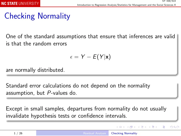
ST 430/514 Introduction to Regression Analysis/Statistics for Management and the Social Sciences II Checking Normality One of the standard assumptions that ensure that inferences are valid is that the random errors = Y E ( Y | x ) are
ST 430/514 Introduction to Regression Analysis/Statistics for Management and the Social Sciences II Checking Normality One of the standard assumptions that ensure that inferences are valid is that the random errors ǫ = Y − E ( Y | x ) are normally distributed. Standard error calculations do not depend on the normality assumption, but P -values do. Except in small samples, departures from normality do not usually invalidate hypothesis tests or confidence intervals. 1 / 26 Residual Analysis Checking Normality
ST 430/514 Introduction to Regression Analysis/Statistics for Management and the Social Sciences II Often, when data are not normal, they show longer/heavier tails. Heavy tails generally make inferences conservative . For instance, a 95% confidence interval actually covers the true parameter value with a probability higher than 95%. Similarly, the Type I error rate in a hypothesis test is less than the nominal α . Conservative inferences are not optimal (for instance, confidence intervals are wider than they need to be), but they are better than anti-conservative. 2 / 26 Residual Analysis Checking Normality
ST 430/514 Introduction to Regression Analysis/Statistics for Management and the Social Sciences II One approach to checking normality is by a hypothesis test: H 0 : ǫ is normally distributed, versus H a : ǫ is not normally distributed. The Shapiro-Wilk test is often recommended. All tests have relatively low power in small samples, and even in moderately large samples. That is, the chance of detecting moderate non-normality is not close to 1. 3 / 26 Residual Analysis Checking Normality
ST 430/514 Introduction to Regression Analysis/Statistics for Management and the Social Sciences II Graphical checks Stem-and-leaf display (semi-graphical) r <- residuals(lm(log(SALARY) ~ EXP + I(EXP^2), workers)) stem(r) produces the display: The decimal point is 1 digit(s) to the left of the | -3 | 54 -2 | 110 -1 | 87665210 -0 | 7776555542221 0 | 01233445788 1 | 045688 2 | 1134566 4 / 26 Residual Analysis Checking Normality
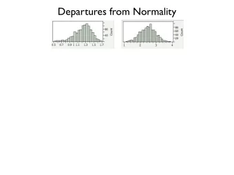
ST 430/514 Introduction to Regression Analysis/Statistics for Management and the Social Sciences II Histogram hist(r) # to match Figure 8.20: hist(r, breaks = seq(from = -0.425, to = 0.425, by = 0.05), freq = FALSE) # overlay a normal curve: curve(dnorm(x, mean = mean(r), sd = sd(r)), col = "red", add = TRUE) Quantile-quantile plot qqnorm(r) # to match Figure 8.22: qqnorm(r, datax = TRUE) Note: The quantile-quantile plot is more useful than the histogram, even with an overlaid normal density. 5 / 26 Residual Analysis Checking Normality
ST 430/514 Introduction to Regression Analysis/Statistics for Management and the Social Sciences II Outliers y i is the i th residual; it has the same units as Y . Recall that ˆ ǫ i = y i − ˆ Residuals are often scaled in some way to make them dimensionless. Terminology varies! Here we follow R ( rstandard() and rstudent() ) and SAS/INSIGHT, not the text. 6 / 26 Residual Analysis Outliers, Leverage, and Influence
ST 430/514 Introduction to Regression Analysis/Statistics for Management and the Social Sciences II Scaled residual (“standardized” residual in the text): scaled residual z i = ˆ ǫ i s = y i − ˆ y i . s Rule of thumb If | z i | > 3, the i th observation is an outlier . Equivalently, | y i − ˆ y i | > 3 s , a “3- σ event”. 7 / 26 Residual Analysis Outliers, Leverage, and Influence
ST 430/514 Introduction to Regression Analysis/Statistics for Management and the Social Sciences II The “hat” matrix Each observation contributes to the value of ˆ β ; in matrix notation, β = ( X ′ X ) − 1 X ′ y . ˆ So it also contributes to the predicted values: β = X ( X ′ X ) − 1 X ′ y = Hy , y = X ˆ ˆ where H = X ( X ′ X ) − 1 X ′ is the hat matrix. H “puts the hat on y ”. 8 / 26 Residual Analysis Outliers, Leverage, and Influence
ST 430/514 Introduction to Regression Analysis/Statistics for Management and the Social Sciences II The residuals are ˆ ǫ = y − ˆ y = ( I − H ) y and consequently (with some matrix algebra) ǫ i ) = σ 2 (1 − h i ) var (ˆ where h i is the i th diagonal entry in H . The ˆ ǫ i y i − ˆ y i z i standardized residual z ∗ s √ 1 − h i s √ 1 − h i √ 1 − h i i = = = (“studentized” residual in the text) is adjusted for these different variances. We can also use the rule of thumb with standardized residuals: if i | > 3, the i th observation is an outlier. | z ∗ 9 / 26 Residual Analysis Outliers, Leverage, and Influence
ST 430/514 Introduction to Regression Analysis/Statistics for Management and the Social Sciences II Example Fast food data with a data-entry error: fast <- read.table("Text/Exercises&Examples/FASTFOOD.txt", header = TRUE) fastBad <- fast fastBad[13, "SALES"] <- 82 lBad <- lm(SALES ~ factor(CITY) + TRAFFIC, fastBad) plot(lBad) Note that the last three plots use standardized residuals z ∗ i , so the rule of thumb is easy to use. An outlier needs careful scrutiny, to distinguish bad data from unusual data. 10 / 26 Residual Analysis Outliers, Leverage, and Influence
ST 430/514 Introduction to Regression Analysis/Statistics for Management and the Social Sciences II Leverage Recall that ˆ y = Hy , where H is the hat matrix: n � y i = ˆ h i , j y j . j =1 The diagonal entry h i , i = h i is the weight attached to y i itself in computing ˆ y i . The diagonal entry h i is defined to be the leverage of the i th observation. Leverage measures the contribution of y i to its predicted value ˆ y i . 11 / 26 Residual Analysis Outliers, Leverage, and Influence
ST 430/514 Introduction to Regression Analysis/Statistics for Management and the Social Sciences II Leverage satisfies 0 < h i ≤ 1; the average leverage is always h = p ¯ n , where p = k + 1 is the number of model parameters (including the intercept). In many designed experiments, all observations have the same leverage: h i ≡ ¯ h ; in observational studies, leverage can vary widely. Rule of thumb h , the i th observation is a leverage point. If h i > 2¯ In the fourth residual plot, the standardized residuals are plotted against leverage. 12 / 26 Residual Analysis Outliers, Leverage, and Influence
ST 430/514 Introduction to Regression Analysis/Statistics for Management and the Social Sciences II Influence An observation can be a leverage point but not have a great influence on ˆ β . ( i ) for the parameter estimates when the i th observation is Write ˆ β omitted. ( i ) is very different from ˆ β , the i th observation has high influence . If ˆ β 13 / 26 Residual Analysis Outliers, Leverage, and Influence
ST 430/514 Introduction to Regression Analysis/Statistics for Management and the Social Sciences II ( i ) − ˆ One measure of the magnitude of ˆ β β is Cook’s distance, � 2 � � n y ( i ) ˆ − ˆ y j j =1 j D i = ps 2 ( i ) − ˆ ( i ) − ˆ � ′ � � � ˆ ˆ ( X ′ X ) β β β β = ps 2 y ( i ) where ˆ y j is the usual predicted value of y j and ˆ is the predicted j ( i ) . value using ˆ β 14 / 26 Residual Analysis Outliers, Leverage, and Influence
ST 430/514 Introduction to Regression Analysis/Statistics for Management and the Social Sciences II It can be shown that D i = z 2 2 � � � � h i = z ∗ h i i i . (1 − h i ) 2 1 − h i p p where z i is the scaled residual, z ∗ i is the standardized residual, and h i is the leverage. If the i th observation has a large standardized residual z ∗ i and high leverage h i , Cook’s distance D i will be large. Rule of thumb If D i > 1, the i th observation is highly influential . 15 / 26 Residual Analysis Outliers, Leverage, and Influence
ST 430/514 Introduction to Regression Analysis/Statistics for Management and the Social Sciences II Note Some statisticians suggest using the median of the F -distribution with p and n − p degrees of freedom as the threshold for being “highly influential”. If p < n / 2, this is less than 1, but often close. Others prefer a yet more stringent threshold of 4 / n . A threshold of 1 is the simplest rule, and is recommended. The fourth residual plot shows contours of Cook’s distance, so the rule of thumb is easy to use. 16 / 26 Residual Analysis Outliers, Leverage, and Influence
ST 430/514 Introduction to Regression Analysis/Statistics for Management and the Social Sciences II Detecting Correlation Time series data Regression models are sometimes used with responses Y 1 , Y 2 , . . . , Y n that are collected over time. Often one response is similar to the immediately preceding responses, which means that they are correlated . Since standard errors are usually calculated on the assumption of zero correlation, they can be quite incorrect, often too small by a factor of 2 or more. 17 / 26 Residual Analysis Detecting Correlation
ST 430/514 Introduction to Regression Analysis/Statistics for Management and the Social Sciences II When such serial correlation is present, both the estimation procedure (least squares) and the calculation of standard errors need to be modified. First we need to know when significant correlation is present. Durbin-Watson test The widely available Durbin-Watson test was developed by Jim Durbin and Geof Watson. It is based on the statistic � n ǫ i − 1 ) 2 i =2 (ˆ ǫ i − ˆ d = . � n ǫ 2 i =1 ˆ i 18 / 26 Residual Analysis Detecting Correlation
Recommend
More recommend
Explore More Topics
Stay informed with curated content and fresh updates.
