CHARMM on the Open Science Grid Tim Miller Laboratory of - PowerPoint PPT Presentation
CHARMM on the Open Science Grid Tim Miller Laboratory of Computational Biology Molecular Simulation and CHARMM CHARMM (Chemistry at Harvard Macromolecular Mechanics) is a widely used program for modeling, simulation, and analysis of
CHARMM on the Open Science Grid Tim Miller Laboratory of Computational Biology
Molecular Simulation and CHARMM ● CHARMM (Chemistry at Harvard Macromolecular Mechanics) is a widely used program for modeling, simulation, and analysis of biological macromolecules. ● The widest use of the program has been for molecular dynamics (MD) simulations. ● In “classical” MD, atoms (including those in solvent) are described explicitly by a force field (CHARMM27) that gives the energy of bonds, angles, dihedral angles, van der Waals forces, etc. ● The force field is used to numerically integrate over Newton's second law of motion to produce updated positions of the atoms.
Issues with Molecular Dynamics On a single core of a 2.33 GHz Intel Clovertown it takes ● almost 10 minutes to simulate 1 picosecond of a moderate sized system. ● At this rate it would take nearly 20 years to run dynamics for 1 μs. And this is without using quantum mechanics based methods. At optimal scaling, we can reduce the ● time by around a factor of 8, which brings us down to 2.5 years. ● Many biologically important processes such as protein folding enzyme catalysis, and conformational rearrangement take place on 1 μs time scales.
More on Molecular Dynamics ● A key goal of an MD simulation is to get a statistical sample over the entire conformation space, but because simulation is so expensive computationally we often do not get this sampling. ● The Langevin equation is often used to maintain a constant temperature throughout the simulation; this is called Langevin dynamics (LD). ● Self-guiding can be added to simulations to enhance the efficiency of conformational searching. ● Self-guided Langevin Dynamics (SGLD) is a relatively new method that combines the LD with self-guiding.
Why use the OSG? Many biological processes are statistical in nature. • Simulations of such processes parallelize naturally because many independent jobs must be run. Performance of multiple simulations on OSG will help with: • Accuracy • Sampling necessary for calculation of experimental observables • Simulate mutants, compare their behaviour and compare with experiments • Test several force-fields - different force-fields may produce different results Describing long timescale processes ( μ s and longer) • • Run large number of simulations (increase probability of observation of important events) • Test different “alternative” methods
Example problem: hydration of the interior of Staphylococcal Nuclease The presence of water in the interior of a protein can affect its role in various biological processes. Staphylococcal Nuclease (SN) is an enzyme that cleaves phosphodiester bonds in nucleic acids. For SN, structure data obtained at different temperatures disagrees on the presence and number of waters at the Glu-66 sidechain. LD simulations can help solve this puzzle.
Hydration of SN (continued) ● Two different conformations the Glu-66 sidechain have been found by simulation, straight and twisted. ● When the sidechain appears straight and extended, 1 or 2 waters are associated with it. When it is twisted back into the protein core, there are no waters. ● The straight conformation occurs most often in simulation, and it is the only one detected by crystallographers. ● A key question is how can we know exactly if and how many waters are present.
Our approach to the problem Previously we performed 10 x 10 ns long simulations, varying the initial velocities of each. This did not yield sufficient statistics to determine the populations of the two conformations! Since observed conformations seem to depend on initial velocities, we decided to run a very large number of shorter (2 ns) simulations. We wanted to vary initial velocities, so for each conformation we ran 40 x 2 ns dynamics simulations, for a total computing time of around 42,000 CPU hours!
What we wanted to test ● Initial conditions: We wanted to see if the results made a difference if we started the structures dehydrated as opposed to hydrated. ● Differences between LD and SGLD: SGLD should in theory give more “flips” between conformations since it samples more efficiently. ● For each of the forty simulations per structure, we ran both LD and SGLD as shown below and observed both the number of waters associated with Glu-66 and the conformation of the sidechain. Number of 2 ns simulations Hydrated Dehydrated LD SGLD LD SGLD 40 40 40 40
Description of the Workflow ● The initial structures were first heated for 100,000 steps (100 ps). ● Then they were equilibrated for 100 ps. ● The two nanoseconds (2 million steps) of dynamics were run. ● The number of waters and the dihedral angle of the Glu-66 residue was extracted from the trajectory and statistics were collected. ● Due to runtime length restrictions at OSG sites, we decided to keep each individual grid job to 50,000 steps (which takes about 12 hours to run on a typical grid node). The image to the right shows two “threads” with many “waves” (individual jobs).
Software set up We need to run a lot of different jobs in order, i.e. a workflow. We use our own software to keep track of the jobs and PanDA/AutoPilot for submission and monitoring.
What the user must do 1. Create CHARMM input scripts for all the various types of jobs to be run. 2. Prepare the structure files and other needed inputs to CHARMM (e.g. topology and parameter files). 3. Package all of these up in a tarball. 4. Write out the workflow and edit shell scripts to point to correct data repositories. 5. Start the executor program. 6. Watch the result files roll in and keep an eye on the logs for problems. 7. If necessary, edit and restart the workflow,
Example Workflow Script JOB heat USE heat.inp heat REQUIRES [NONE NONE] JOB heat2 USE heat2.inp heat2 JOB eq USE eq.inp eq*2 JOB md USE run.inp BRANCH A APPENDPARAMS G=0 JOB analp USE anal_phipsi.inp md*20 JOB analw USE anal_water.inp analp REQUIRES [ALLDONE .res,.trj] PRODUCES # section 2: threads [.dih1,.dih2] NTHREADS 30 analw REQUIRES [ALLDONE THREADPARAMS 'I=[threadid]' .res,.trj] PRODUCES [.wat] BRANCH B APPENDPARAMS G=1 # section 3: Default input md*20 requirement and output production analp REQUIRES [ALLDONE REQDEFAULT [PREVWAVE .res] .res,.trj] PRODUCES PRODEFAULT [.res,.trj,.pdb,.log] [.dih1,.dih2] analw REQUIRES [ALLDONE # section 3: order .res,.trj] PRODUCES [.wat] # The ONLY keywords are END # BRANCH ... REJOIN # TEST ... ENDTEST # LABEL, RESULT, ELSE BEGIN
Our own grid executor! We designed and built software called a grid executor to submit and manage jobs on our behalf. It is written in Python and runs as a daemon, submitting jobs and checking for their output. If a job does not return a result within a set period of time, it is resubmitted. The executor was inspired by DAGMAN for Condor. Jobs can have multiple dependencies and require different inputs and output. The executor is not in any way tied to CHARMM.
What happens on the grid stays on the grid (or not) ● The grid executor submits jobs when the necessary prerequisite jobs have been run. ● The grid jobs are custom written Python scripts, which are responsible for the following tasks: 1. Downloading a tarball containing the CHARMM binary and necessary input scripts and support files. 2. Getting a list of prerequisites and obtaining them from the data store. 3. Running CHARMM with the proper command line arguments and input script. 4. Making sure CHARMM completes OK and then sending back the results.
Job submission and monitoring We use PanDA for job submission and monitoring. This goes us nice management tools and a Python API for defining jobs. Also, PanDA is integrated with AutoPilot which ensures (as much as possible) that remote nodes are able to run the job before it is started.
Basic Results of Simulations ● We observed more straight than twisted conformations, which agrees with previous simulations. ● The two systems are still equilibrating, i.e. they have not settled into their final stable conformations. Therefore the results given are qualitative, not quantitative. ● However, the results appear to be converging (i.e. the effect of the initial hydration state becomes less significant over time). ● We confirmed that the straight conformation is more hydrated than the twisted one. ● We found that during the 2 nd ns, water molecules can become associated with the Glu-66 sidechain even when it is in the twisted state.
Effect of Dehydration ● The initial hydration state dramatically affects the results. ● The state that is initially hydrated prefers the straight conformation ~ 20% more frequently than the initially dehydrated state. ● The conformational switch from straight into twisted often occurs when the straight sidechain is dehydrated. ● Flips from straight into twisted occur after a drop in hydration (as shown in the figure). ● When structures flip from twisted to straight, average number of waters present increases more gradually.
Recommend
More recommend
Explore More Topics
Stay informed with curated content and fresh updates.


