Chapter 9: Rule Mining 9.1 OLAP 9.2 Association Rules 9.3 Iceberg - PowerPoint PPT Presentation

Chapter 9: Rule Mining 9.1 OLAP 9.2 Association Rules 9.3 Iceberg Queries 9-1 IRDM WS 2005

9.1 OLAP: Online Analytical Processing Mining business data for interesting facts and decision support (CRM, cross-selling, fraud, trading/usage patterns and exceptions, etc.) • with data from different production sources integrated into data warehouse , • often with data subsets extracted and transformed into data cubes Monitoring & Administration Metadata Repository OLAP Servers OLAP Data Warehouse External Extract sources Transform Query/Reporting Load Operational Serve DBS Data Mining Data sources Front-End Tools Data Marts 9-2 IRDM WS 2005

Typical OLAP (Decision Support) Queries • What were the sales volumes by region and product category for the last year? • How did the share price of computer manufacturers correlate with quarterly profits over the past 10 years? • Which orders should we fill to maximize revenues? • Will a 10% discount increase sales volume sufficiently? • Which products should we advertise to the various categories of our customers? • Which of two new medications will result in the best outcome: higher recovery rate & shorter hospital stay? • Which ads should be on our Web site to which category of users? • How should we personalize our Web site based on usage logs? • Which symptoms indicate which disease? • Which genes indicate high cancer risk? 9-3 IRDM WS 2005

Data Warehouse with Star Schema Product Order ProdNo OrderNo ProdName OrderDate ProdDescr Fact table Category CategoryDescr Customer OrderNo UnitPrice SalespersonID CustomerNo QOH CustomerNo CustomerName ProdNo Date CustomerAddress DateKey City CityName DateKey Quantity Date Salesperson TotalPrice Month Year SalespersonID SalespersonName City City CityName Quota State Country data often comes from different sources of different organizational units → data cleaning is a major problem 9-4 IRDM WS 2005

Data Warehouse with Snowflake Schema Product Category Order ProdNo OrderNo CategoryName ProdName OrderDate CategoryDescr ProdDescr Fact table Category UnitPrice Customer OrderNo QOH SalespersonID CustomerNo CustomerNo CustomerName DateKey Year Date Month CustomerAddress CityName City ProdNo DateKey Year Month Quantity Date Year Salesperson TotalPrice Month SalespersonID City State SalespesonName CityName City StateName State Quota Country 9-5 IRDM WS 2005

Data Cube • organize data (conceptually) into a multidimensional array • analysis operations (OLAP algebra, integrated into SQL): roll-up/drill-down, slice&dice (sub-cubes), pivot (rotate), etc. Example: sales volume as a function of product, time, geography y y t Fact data: sales volume in $100 t LA i i C C SF Dimensions: NY 117 Product, City, Date 10 Juice Attributes: Product Product Cola 50 Product (prodno, price, ...) Milk 20 Attribute Hierarchies and Lattices: Cream 12 Industry Country Year Toothpaste 15 Soap 10 Category State Quarter 1 2 3 4 5 6 7 Product City Month Week Date Date for high dimensionality: Date cube could be approximated by Bayesian net 9-6 IRDM WS 2005

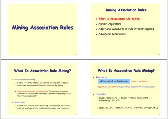
9.2 Association Rules given: a set of items I = {x1, ..., xm} a set (bag) D={t1, ..., tn} of item sets (transactions) ti = {xi 1 , ..., xi k } ⊆ I wanted: rules of the form X ⇒ Y with X ⊆ I and Y ∈ I such that • X is sufficiently often a subset of the item sets ti and • when X ⊆ ti then most frequently Y ∈ ti holds, too. support (X ⇒ Y) = P[XY] = relative frequency of item sets that contain X and Y confidence (X ⇒ Y) = P[Y|X] = relative frequency of item sets that contain Y provided they contain X support is usually chosen in the range of 0.1 to 1 percent, confidence (aka. strength) in the range of 90 percent or higher 9-7 IRDM WS 2005

Association Rules: Example Market basket data („sales transactions“): t1 = {Bread, Coffee, Wine} t2 = {Coffee, Milk} t3 = {Coffee, Jelly} t4 = {Bread, Coffee, Milk} t5 = {Bread, Jelly} t6 = {Coffee, Jelly} t7 = {Bread, Jelly} t8 = {Bread, Coffee, Jelly, Wine} t9 = {Bread, Coffee, Jelly} support (Bread ⇒ Jelly) = 4/9 confidence (Bread ⇒ Jelly) = 4/6 support (Coffee ⇒ Milk) = 2/9 confidence (Coffee ⇒ Milk) = 2/7 support (Bread, Coffee ⇒ Jelly) = 2/9 confidence (Bread, Coffee ⇒ Jelly) = 2/4 9-8 IRDM WS 2005

Apriori Algorithm: Idea and Outline Idea and outline: • proceed in phases i=1, 2, ..., each making a single pass over D, and generate rules X ⇒ Y with frequent item set X (sufficient support) and |X|=i in phase i; • use phase i-1 results to limit work in phase i: antimonotonicity property (downward closedness): for i-item-set X to be frequent, each subset X‘ ⊆ X with |X‘|=i-1 must be frequent, too • generate rules from frequent item sets; • test confidence of rules in final pass over D Worst-case time complexity is exponential in I and linear in D*I, but usual behavior is linear in D (detailed average-case analysis is very difficult) 9-9 IRDM WS 2005

Apriori Algorithm: Pseudocode procedure apriori (D, min-support): L 1 = frequent 1-itemsets(D); for (k=2; L k-1 ≠ ∅ ; k++) { C k = apriori-gen (L k-1 , min-support); for each t ∈ D { // linear scan of D C t = subsets of t that are in C k ; for each candidate c ∈ C t {c.count++}; }; L k = {c ∈ C k | c.count ≥ min-support}; }; return L = ∪ k L k ; // returns all frequent item sets procedure apriori-gen (L k-1 , min-support): C k = ∅ : for each itemset x 1 ∈ L k-1 { for each itemset x 2 ∈ L k-1 { if x 1 and x 2 have k-2 items in common and differ in 1 item // join { x = x 1 ∪ x 2 ; if there is a subset s ⊆ x with s ∉ L k-1 {disregard x;} // infreq. subset else add x to C k ; }; }; }; return C k 9-10 IRDM WS 2005

Algorithmic Extensions and Improvements • hash-based counting (computed during very first pass): map k-itemset candidates (e.g. for k=2) into hash table and maintain one count per cell; drop candidates with low count early • remove transactions that don‘t contain frequent k-itemset for phases k+1, ... • partition transactions D: an itemset is frequent only if it is frequent in at least one partition • exploit parallelism for scanning D • randomized (approximative) algorithms : find all frequent itemsets with high probability (using hashing etc.) • sampling on a randomly chosen subset of D ... mostly concerned about reducing disk I/O cost (for TByte databases of large wholesalers or phone companies) 9-11 IRDM WS 2005

Extensions and Generalizations of Assocation Rules • quantified rules : consider quantitative attributes of item in transactions (e.g. wine between $20 and $50 ⇒ cigars, or age between 30 and 50 ⇒ married, etc.) • constrained rules : consider constraints other than count thresholds, e.g. count itemsets only if average or variance of price exceeds ... • generalized aggregation rules : rules referring to aggr. functions other than count, e.g., sum(X.price) ⇒ avg(Y.age) • multilevel association rules : considering item classes (e.g. chips, peanuts, bretzels, etc. belonging to class snacks) • sequential patterns (e.g. an itemset is a customer who purchases books in some order, or a tourist visiting cities and places) • from strong rules to interesting rules : consider also lift (aka. interest) of rule X ⇒ Y: P[XY] / P[X]P[Y] • correlation rules • causal rules 9-12 IRDM WS 2005

Correlation Rules example for strong, but misleading association rule: tea ⇒ coffee with confidence 80% and support 20% but support of coffee alone is 90%, and of tea alone it is 25% → tea and coffee have negative correlation ! consider contingency table (assume n=100 transactions): ¬ T T C 20 70 90 → {T, C} is a frequent and correlated item set ¬ C 5 5 10 25 75 2 ∧ − ( freq ( X Y ) freq ( X ) freq ( Y ) / n ) 2 χ = ( C , T ) ( ∑ ∑ freq ( X ) freq ( Y ) / n ∈ ∈ X { C , C } Y { T , T } correlation rules are monotone (upward closed): if the set X is correlated then every superset X‘ ⊇ X is correlated, too. 9-13 IRDM WS 2005

Correlation Rules example for strong, but misleading association rule: tea ⇒ coffee with confidence 80% and support 20% but support of coffee alone is 90%, and of tea alone it is 25% → tea and coffee have negative correlation ! consider contingency table (assume 100 transactions): ¬ T E[C]=0.9 T E[T]=0.25 C 20 70 90 E[(T-E[T])2]=1/4 * 9/16 +3/4 * 1/16= 3/16=Var(T) E[(C-E[C])2]=9/10 * 1/100 +1/10 * 1/100 = 9/100=Var(C) ¬ C 5 5 10 E[(T-E[T])(C-E[C])]= 2/10 * 3/4 * 1/10 - 7/10 * 1/4 * 1/10 25 75 - 5/100 * 3/4 * 9/10 + 5/100 * 1/4 * 9/10 = 60/4000 – 70/4000 – 135/4000 + 45/4000 = - 1/40 = Cov(C,T) ρ (C,T) = - 1/40 * 4/sqrt(3) * 10/3 ≈ -1/(3*sqrt(3)) ≈ - 0.2 9-14 IRDM WS 2005