Chapter 8 In the Solow model of Chapter 7, the production - PDF document

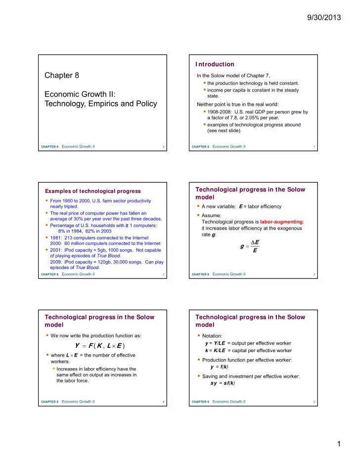
9/30/2013 I ntroduction Chapter 8 In the Solow model of Chapter 7,  the production technology is held constant.  income per capita is constant in the steady Economic Growth II: state. Technology Empirics and Policy Technology, Empirics and Policy Neither point is true in the real world: N ith i t i t i th l ld  1908-2008: U.S. real GDP per person grew by a factor of 7.8, or 2.05% per year.  examples of technological progress abound (see next slide). Economic Growth II Economic Growth II CHAPTER 8 0 CHAPTER 8 1 Technological progress in the Solow Examples of technological progress model  From 1950 to 2000, U.S. farm sector productivity  A new variable: E = labor efficiency nearly tripled.  The real price of computer power has fallen an  Assume: average of 30% per year over the past three decades. Technological progress is labor-augmenting :  Percentage of U.S. households with ≥ 1 computers: it increases labor efficiency at the exogenous y g 8% in 1984 8% in 1984, 62% in 2003 62% in 2003 rate g :  1981: 213 computers connected to the Internet  E 2000: 60 million computers connected to the Internet  g  2001: iPod capacity = 5gb, 1000 songs. Not capable E of playing episodes of True Blood . 2009: iPod capacity = 120gb, 30,000 songs. Can play episodes of True Blood . Economic Growth II Economic Growth II CHAPTER 8 2 CHAPTER 8 3 Technological progress in the Solow Technological progress in the Solow model model  We now write the production function as:  Notation: y = Y/LE = output per effective worker   Y F K ( , L E ) k = K/LE = capital per effective worker  where L  E = the number of effective  Production function per effective worker: workers. y = f ( k )  Increases in labor efficiency have the same effect on output as increases in  Saving and investment per effective worker: the labor force. sy = sf ( k ) Economic Growth II Economic Growth II CHAPTER 8 4 CHAPTER 8 5 1

9/30/2013 Technological progress in the Solow Technological progress in the Solow model model  k = s f ( k )  (  + n + g ) k (  + n + g ) k = break-even investment: Investment, break-even the amount of investment necessary investment (  + n + g ) k to keep k constant. Consists of: Consists of: sf(k) ( )   k to replace depreciating capital  nk to provide capital for new workers  gk to provide capital for the new “effective” workers created by technological progress Capital per k * worker, k Economic Growth II Economic Growth II CHAPTER 8 6 CHAPTER 8 7 Steady-state growth rates in the The Golden Rule with technological Solow model with tech. progress progress Steady-state To find the Golden Rule capital stock, Variable Symbol express c * in terms of k * : growth rate In the Golden Capital per  = y * c * i * k = K / ( L  E ) 0 Rule steady state, effective worker  (  + n + g ) k * (  + n + g ) k the marginal the marginal = f ( k * ) f ( k ) Output per product of capital y = Y / ( L  E ) 0 c * is maximized when effective worker net of depreciation MPK =  + n + g equals the ( Y / L ) = y  E Output per worker g pop. growth rate or equivalently, plus the rate of MPK   = n + g tech progress. Y = y  E  L Total output n + g Economic Growth II Economic Growth II CHAPTER 8 8 CHAPTER 8 9 Growth empirics: Balanced growth Growth empirics: Convergence  Solow model’s steady state exhibits  Solow model predicts that, other things equal, balanced growth - many variables grow “poor” countries (with lower Y / L and K / L ) should at the same rate. grow faster than “rich” ones.  Solow model predicts Y / L and K / L grow at the  If true, then the income gap between rich & poor same rate ( g ) so K / Y should be constant same rate ( g ), so K / Y should be constant. countries would shrink over time, causing living This is true in the real world. standards to “converge.”  Solow model predicts real wage grows at same  In real world, many poor countries do NOT grow rate as Y / L , while real rental price is constant. faster than rich ones. Does this mean the Solow Also true in the real world. model fails? Economic Growth II Economic Growth II CHAPTER 8 10 CHAPTER 8 11 2

9/30/2013 Growth empirics: Convergence Growth empirics: Convergence  What the Solow model really predicts is  Solow model predicts that, other things equal, conditional convergence - countries converge “poor” countries (with lower Y / L and K / L ) should to their own steady states, which are determined grow faster than “rich” ones. by saving, population growth, and education.  No, because “other things” aren’t equal.  This prediction comes true in the real world.  In samples of countries with similar savings & pop. growth rates, income gaps shrink about 2% per year.  In larger samples, after controlling for differences in saving, pop. growth, and human capital, incomes converge by about 2% per year. Economic Growth II Economic Growth II CHAPTER 8 12 CHAPTER 8 13 Growth empirics: Factor accumulation Growth empirics: Factor accumulation vs. production efficiency vs. production efficiency  Differences in income per capita among countries  Possible explanations for the correlation can be due to differences in: between capital per worker and production efficiency: 1. capital – physical or human – per worker  Production efficiency encourages capital 2. the efficiency of production (th (the height of the production function) h i ht f th d ti f ti ) accumulation.  Studies:  Capital accumulation has externalities that  Both factors are important. raise efficiency.  The two factors are correlated: countries with  A third, unknown variable causes higher physical or human capital per worker also capital accumulation and efficiency to be tend to have higher production efficiency. higher in some countries than others. Economic Growth II Economic Growth II CHAPTER 8 14 CHAPTER 8 15 Growth empirics: Growth empirics: Production efficiency and free trade Production efficiency and free trade  Since Adam Smith, economists have argued that  To determine causation, Frankel and Romer free trade can increase production efficiency and exploit geographic differences among countries: living standards.  Some nations trade less because they are farther  Research by Sachs & Warner: from other nations, or landlocked.  Such geographical differences are correlated with  Such geographical differences are correlated with Average annual growth rates, 1970-89 trade but not with other determinants of income.  Hence, they can be used to isolate the impact of open closed trade on income. developed nations 2.3% 0.7%  Findings: increasing trade/GDP by 2% causes developing nations 4.5% 0.7% GDP per capita to rise 1%, other things equal. Economic Growth II Economic Growth II CHAPTER 8 16 CHAPTER 8 17 3

9/30/2013 Policy issues: Policy issues Evaluating the rate of saving  Are we saving enough? Too much?  Use the Golden Rule to determine whether the U.S. saving rate and capital stock are too  What policies might change the saving rate? high, too low, or about right.  How should we allocate our investment between  If ( MPK   ) > ( n + g ), privately owned physical capital, public U S is below the Golden Rule steady state U.S. is below the Golden Rule steady state infrastructure, and “human capital”? and should increase s .  How do a country’s institutions affect production  If ( MPK   ) < ( n + g ), efficiency and capital accumulation? U.S. economy is above the Golden Rule steady  What policies might encourage faster state and should reduce s . technological progress? Economic Growth II Economic Growth II CHAPTER 8 18 CHAPTER 8 19 Policy issues: Policy issues: Evaluating the rate of saving Evaluating the rate of saving To estimate ( MPK   ), use three facts about the 1. k = 2.5 y U.S. economy: 2.  k = 0.1 y 1. k = 2.5 y 3. MPK  k = 0.3 y The capital stock is about 2.5 times one year’s GDP. GDP To determine  , divide 2 by 1 : 2.  k = 0.1 y About 10% of GDP is used to replace depreciating   0.1 0.1 k y     0.04 capital. 2.5 2.5 k y 3. MPK  k = 0.3 y Capital income is about 30% of GDP. Economic Growth II Economic Growth II CHAPTER 8 20 CHAPTER 8 21 Policy issues: Policy issues: Evaluating the rate of saving Evaluating the rate of saving 1. k = 2.5 y  From the last slide: MPK   = 0.08 2.  k = 0.1 y  U.S. real GDP grows an average of 3% per year, so n + g = 0.03 3. MPK  k = 0.3 y  Thus Thus, To determine MPK, divide 3 by 1 : MPK   = 0.08 > 0.03 = n + g  Conclusion: MPK  0.3  0.3 k y    MPK 0.12 2.5 k y 2.5 The U.S. is below the Golden Rule steady state: Increasing the U.S. saving rate would increase Hence, MPK   = 0.12  0.04 = 0.08 consumption per capita in the long run. Economic Growth II Economic Growth II CHAPTER 8 22 CHAPTER 8 23 4