Chapter 7: Rapid alignment methods: FASTA and BLAST The biological - PowerPoint PPT Presentation
Chapter 7: Rapid alignment methods: FASTA and BLAST The biological problem l Search strategies l FASTA l BLAST l Introduction to bioinformatics, Autumn 2007 83 The biological problem Global and local alignment algoritms are slow in
Chapter 7: Rapid alignment methods: FASTA and BLAST The biological problem l Search strategies l FASTA l BLAST l Introduction to bioinformatics, Autumn 2007 83
The biological problem • Global and local alignment algoritms are slow in practice • Consider the scenario of aligning a query sequence against a large database of sequences – New sequence with For instance, the size of NCBI • unknown function GenBank in January 2007 was 65,369,091,950 bases (61,132,599 sequences) Introduction to bioinformatics, Autumn 2007 84
Problem with large amount of sequences Exponential growth in both number and total length of l sequences Possible solution: Compare against model organisms l only With large amount of sequences, changes are that l matches occur by random − Need for statistical analysis Introduction to bioinformatics, Autumn 2007 85
Application of sequence alignment: shotgun sequencing Shotgun sequencing is a method for sequencing l whole-organism genomes − First, a large number of short sequences (~500-1000 bp), or reads are generated from the genome − Reads are contiguous subsequences (substrings) of the genome − Due to sequencing errors and repetitions in the reads, the genome has be covered multiple times by reads Introduction to bioinformatics, Autumn 2007 86
Shotgun sequencing Original genome sequence … … Reads Non-overlapping Overlapping reads read => Contig Ordering of the reads is initially unknown l Overlaps resolved by aligning the reads l In a 3x10 9 bp genome with 500 bp reads and 5x coverage, there l are ~10 7 reads and ~10 7 (10 7 -1)/2 = ~5x10 13 pairwise sequence comparisons Introduction to bioinformatics, Autumn 2007 87
Shotgun sequencing Original genome sequence … … Reads Non-overlapping Overlapping reads read => Contig ~5x10 13 pairwise sequence comparisons l Recall that local alignment takes O(nm) time, where n and m are l sequence lengths Already with n=m=500, the computation cost is prohibitive l Introduction to bioinformatics, Autumn 2007 88
Search strategies How to speed up the computation? l − Find ways to limit the number of pairwise comparisons Compare the sequences at word level to find out l common words − Word means here a k-tuple (or a k-word), a substring of length k Introduction to bioinformatics, Autumn 2007 89
Analyzing the word content Example query string I: TGATGATGAAGACATCAG l For k = 8, the set of k-tuples of I is l TGATGATG GATGATGA ATGATGAA TGATGAAG … GACATCAG Introduction to bioinformatics, Autumn 2007 90
Analyzing the word content There are n-k+1 k-tuples in a string of length n l If at least one word of I is not found from another string l J, we know that I differs from J Need to consider statistical significance: I and J l might share words by chance only Let n=|I| and m=|J| l Introduction to bioinformatics, Autumn 2007 91
Word lists and comparison by content The k-words of I can be arranged into a table of word l occurences L w (I) Consider the k-words when k=2 and I=GCATCGGC: l GC, CA, AT, TC, CG, GG, GC AT: 3 CA: 2 CG: 5 GC: 1, 7 Start indecies of k-word GC in I GG: 6 Building L w (I) takes O(n) time TC: 4 Introduction to bioinformatics, Autumn 2007 92
Common k-words Number of common k-words in I and J can be l computed using L w (I) and L w (J) For each word w in I, there are |L w (J)| occurences in J l Therefore I and J have l common words This can be computed in O(n + m + 4 k ) time l − O(n + m) time to build the lists − O(4 k ) time to calculate the sum Introduction to bioinformatics, Autumn 2007 93
Common k-words I = GCATCGGC l J = CCATCGCCATCG l L w (I) L w (J) Common words AT: 3 AT: 3, 9 2 CA: 2 CA: 2, 8 2 CC: 1, 7 0 CG: 5 CG: 5, 11 2 GC: 1, 7 GC: 6 2 GG: 6 0 TC: 4 TC: 4, 10 2 10 in total Introduction to bioinformatics, Autumn 2007 94
Properties of the common word list Exact matches can be found using binary search (e.g., where l TCGT occurs in I?) − O(log 4 k ) time For large k, the table size is too large to compute the common l word count in the previous fashion Instead, an approach based on merge sort can be utilised l (details skipped, see course book) The common k-word technique can be combined with the local l alignment algorithm to yield a rapid alignment approach Introduction to bioinformatics, Autumn 2007 95
Chapter 7: Rapid alignment methods: FASTA and BLAST The biological problem l Search strategies l FASTA l BLAST l Introduction to bioinformatics, Autumn 2007 96
FASTA FASTA is a multistep algorithm for sequence alignment (Wilbur l and Lipman, 1983) The sequence file format used by the FASTA software is widely l used by other sequence analysis software Main idea: l − Choose regions of the two sequences that look promising (have some degree of similarity) − Compute local alignment using dynamic programming in these regions Introduction to bioinformatics, Autumn 2007 97
FASTA outline FASTA algorithm has five steps: l − 1. Identify common k-words between I and J − 2. Score diagonals with k-word matches, identify 10 best diagonals − 3. Rescore initial regions with a substitution score matrix − 4. Join initial regions using gaps, penalise for gaps − 5. Perform dynamic programming to find final alignments Introduction to bioinformatics, Autumn 2007 98
Dot matrix comparisons Word matches in two sequences I and J can be represented as l a dot matrix Dot matrix element (i, j) has ”a dot”, if the word starting at l position i in I is identical to the word starting at position j in J The dot matrix can be plotted for various k l j i I = … ATCGGATCA … J = … TGGTGTCGC … i j Introduction to bioinformatics, Autumn 2007 99
k=1 k=4 Dot matrix (k=1,4,8,16) for two DNA sequences X85973.1 (1875 bp) Y11931.1 (2013 bp) k=8 k=16 Introduction to bioinformatics, Autumn 2007 100
k=1 k=4 Dot matrix (k=1,4,8,16) for two protein sequences CAB51201.1 (531 aa) CAA72681.1 (588 aa) k=8 k=16 Shading indicates now the match score according to a score matrix (Blosum62 here) Introduction to bioinformatics, Autumn 2007 101
Computing diagonal sums We would like to find high scoring diagonals of the dot matrix l Lets index diagonals by the offset, l = i - j l J C C A T C G C C A T C G k=2 G * C * * A * * T * * I C * * G G * Diagonal l = i – j = -6 C Introduction to bioinformatics, Autumn 2007 102
Computing diagonal sums As an example, lets compute diagonal sums for I = l GCATCGGC, J = CCATCGCCATCG, k = 2 1. Construct k-word list L w (J) l 2. Diagonal sums S l are computed into a table, indexed with the l offset and initialised to zero l -10 -9 -8 -7 -6 -5 -4 -3 -2 -1 0 1 2 3 4 5 6 S l 0 0 0 0 0 0 0 0 0 0 0 0 0 0 0 0 0 Introduction to bioinformatics, Autumn 2007 103
Computing diagonal sums 3. Go through k-words of I, look for matches in L w (J) and update l diagonal sums For the first 2-word in I, J GC, L GC (J) = {6}. C C A T C G C C A T C G G * We can then update C * * the sum of diagonal A * * l = i – j = 1 – 6 = -5 to S -5 := S -5 + 1 = 0 + 1 = 1 T * * I C * * G G * C Introduction to bioinformatics, Autumn 2007 104
Computing diagonal sums 3. Go through k-words of I, look for matches in L w (J) and update l diagonal sums Next 2-word in I is CA, J for which L CA (J) = {2, 8}. C C A T C G C C A T C G G * Two diagonal sums are C * * updated: A * * l = i – j = 2 – 2 = 0 S 0 := S 0 + 1 = 0 + 1 = 1 T * * I C * * I = i – j = 2 – 8 = -6 G S -6 := S -6 + 1 = 0 + 1 = 1 G * C Introduction to bioinformatics, Autumn 2007 105
Computing diagonal sums 3. Go through k-words of I, look for matches in L w (J) and update l diagonal sums Next 2-word in I is AT, J for which L AT (J) = {3, 9}. C C A T C G C C A T C G G * Two diagonal sums are C * * updated: A * * l = i – j = 3 – 3 = 0 S 0 := S 0 + 1 = 1 + 1 = 2 T * * I C * * I = i – j = 3 – 9 = -6 G S -6 := S -6 + 1 = 1 + 1 = 2 G * C Introduction to bioinformatics, Autumn 2007 106
Computing diagonal sums After going through the k-words of I, the result is: l -10 -9 -8 -7 -6 -5 -4 -3 -2 -1 0 1 2 3 4 5 6 S l 0 0 0 0 4 1 0 0 0 0 4 1 0 0 0 0 0 J C C A T C G C C A T C G G * C * * A * * T * * I C * * G G * C Introduction to bioinformatics, Autumn 2007 107
Algorithm for computing diagonal sum of scores S l := 0 for all 1 – m � l � n – 1 Compute L w (J) for all words w for i := 1 to n – k – 1 do w := I i I i+1 …I i+k-1 for j � L w (J) do l := i – j S l := S l + 1 Match score is here 1 end end Introduction to bioinformatics, Autumn 2007 108
Recommend
More recommend
Explore More Topics
Stay informed with curated content and fresh updates.




![Geno2pheno[coreceptor] 3 Geno2pheno[454] Geno2pheno[454] fasta-format sff-, or fasta-format](https://c.sambuz.com/491954/geno2pheno-coreceptor-s.webp)
