Chapter 7: Product Differentiation A1. Firms meet only once in the - PDF document
Chapter 7: Product Differentiation A1. Firms meet only once in the market. Relax A2. Products are differentiated. A3. No capacity constraints. Timing: 1. fi rms choose simultaneously their location in the product space, 2. given the location,
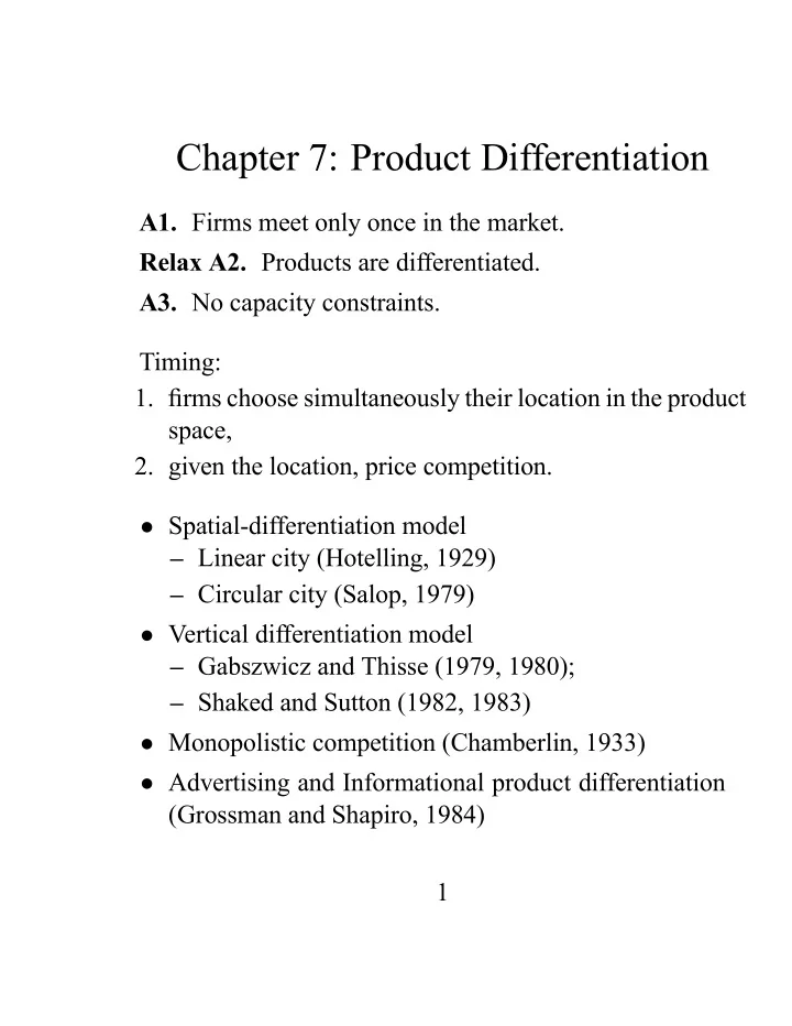
Chapter 7: Product Differentiation A1. Firms meet only once in the market. Relax A2. Products are differentiated. A3. No capacity constraints. Timing: 1. fi rms choose simultaneously their location in the product space, 2. given the location, price competition. • Spatial-differentiation model – Linear city (Hotelling, 1929) – Circular city (Salop, 1979) • Vertical differentiation model – Gabszwicz and Thisse (1979, 1980); – Shaked and Sutton (1982, 1983) • Monopolistic competition (Chamberlin, 1933) • Advertising and Informational product differentiation (Grossman and Shapiro, 1984) 1
1 Spatial Competition 1.1 The linear city (Hotelling, 1929) • Linear city of length 1. • Duopoly with same physical good. • Consumers are distributed uniformly along the city, N = 1 • Quadratic transportation costs t per unit of length. • They consume either 0 or 1 unit of the good. • If locations are given, what is the NE in price? Price Competition Maximal differentiation • 2 shops are located at the 2 ends of the city, shop 1 is at x = 0 and of shop 2 is at x = 1 . c unit cost • p 1 and p 2 are the prices charged by the 2 shops. • Price of going to shop 1 for a consumer at x is p 1 + tx 2 . • Price of going to shop 2 for a cons. at x p 2 + t (1 − x ) 2 . • The utility of a consumer located at x is 2
s − p 1 − tx 2 if he buys from shop 1 s − p 2 − t (1 − x ) 2 if he buys from shop 2 U = otherwise 0 • Assumption: prices are not too high (2 fi rms serve the market) • Demands are D 1 ( p 1 , p 2 ) = p 2 − p 1 + t 2 t D 2 ( p 1 , p 2 ) = p 1 − p 2 + t 2 t • and pro fi t Π i ( p i , p j ) = ( p i − c ) p j − p i + t 2 t • So each fi rm maximizes its pro fi t and the FOC gives p i = p j + t − c for each fi rm i 2 • Prices are strategic complements: ∂ 2 Π i ( p i , p j ) > 0 . ∂ p i ∂ p j 3
• The Nash equilibrium in price is p ∗ i = p ∗ j = c + t • The equilibrium pro fi ts are Π 1 = Π 2 = t 2 Minimal differentiation • 2 shops are located at the same location x o . • p 1 and p 2 are the prices charged by the 2 shops. • Price of going to shop 1 for a consumer at x is p 1 + t ( x o − x ) 2 . • Price of going to shop 2 for a consumer at x is p 2 + t ( x o − x ) 2 . • The consumers compare prices.... Bertrand competition • Nash equilibrium in prices is p ∗ i = p ∗ j = c • and the equilibrium pro fi ts are Π 1 = Π 2 = 0 4
Different locations • 2 shops are located at x = a and of shop 2 is at x = 1 − b where 1 − a − b ≥ 0 . • If a = b = 0 : maximal differentiation • If a + b = 1 : minimal differentiation • p 1 and p 2 are the prices charged by the 2 shops. • Price of going to shop 1 for a consumer at x is p 1 + t ( x − a ) 2 . • Price of going to shop 2 for a consumer at x is p 2 + t (1 − b − x ) 2 . • Thus there exists an indifferent consumer located at e x x − a ) 2 = p 2 + t (1 − b − e x ) 2 p 1 + t ( e 2(1 − a − b ) + 1 − b + a p 2 − p 1 ⇒ e x = 2 • and thus the demand for each fi rm is D 1 ( p 1 , p 2 ) = a + 1 − b − a p 2 − p 1 + 2 2(1 − a − b ) D 2 ( p 1 , p 2 ) = b + 1 − b − a p 1 − p 2 + 2 2(1 − a − b ) 5
• The Nash equilibrium in price is 1 ( a, b ) = c + t (1 − a − b )(1 + a − b p ∗ ) 3 2 ( a, b ) = c + t (1 − a − b )(1 + b − a p ∗ ) 3 • Pro fi ts are Π 1 ( a, b ) = [ p ∗ 1 ( a, b ) − c ] D 1 ( a, p ∗ 1 ( a, b ) , p ∗ 2 ( a, b )) Π 2 ( a, b ) = [ p ∗ 2 ( a, b ) − c ] D 2 ( b, p ∗ 1 ( a, b ) , p ∗ 2 ( a, b )) Product Choice Timing: 1. fi rms choose their location simultaneously 2. given the location, they simultaneously choose prices • Firm 1 chooses a that maximizes Π 1 ( a, b ) ⇒ a ( b ) • Firm 2 chooses b that maximizes Π 2 ( a, b ) ⇒ b ( a ) • and then ( a ∗ , b ∗ ). • What is the optimal choice of location? 6
d Π 1 ( a, b ) = ∂ Π 1 ( a, b ) ∂ a + ∂ Π 1 ( a, b ) + ∂ Π 1 ( a, b ) ∂ p 1 ∂ p 2 da ∂ p 1 ∂ a ∂ p 2 ∂ a where ∂ Π 1 ( a, b ) ∂ p 1 ∂ a = 0 (due to envelope theorem) ∂ p 1 • We can rewrite d Π 1 ( a, b ) 1 ( a, b ) − c ]( ∂ D 1 ( . ) + ∂ D 2 ( . ) ∂ p 2 = [ p ∗ ∂ a ) da ∂ a ∂ p 2 where ∂ D 1 ( . ) 3 − 5 a − b 6(1 − a − b ) Demand Effect (DE) = ∂ a and ∂ D 2 ( . ) ∂ p 2 − 2 + a 3(1 − a − b ) < 0 Strategic Effect (SE) ∂ a = ∂ p 2 Thus, d Π 1 ( a, b ) 1 ( a, b ) − c ]( − 1 − 3 a − b = [ p ∗ 6(1 − a − b )) < 0 da • As a decreases, Π 1 ( a, b ) increases. Result The Nash Equilibrium is such that there is maximal differentiation , i.e. ( a ∗ = 0 , b ∗ = 0) 7
• 2 effects may work in opposite direction – SE < 0 (always): price competition pushes fi rms to locate as far as possible. – DE can be > 0 if a ≤ 1 / 2 , to increase market share , given prices, pushes fi rms toward the center. – But overall SE > DE, and they locate at the two extremes. 1.1.1 Social planner • Minimizes the average transportation costs. • Thus locates fi rms at a s = 1 4 , b s = 1 4 Result Maximal differentiation yields too much product differentiation compared to what is socially optimal. 8
1.2 The circular city (Salop, 1979) • circular city • large number of identical potential fi rms • Free entry condition • consumers are located uniformly on a circle of perimeter equal to 1 • Density of unitary around the circle. • Each consumer has a unit demand • unit transportation cost • gross surplus s . • f fi xed cost of entry • marginal cost is c • Firm i ’s pro fi t is ( ( p i − c ) D i − f if entry Π i = otherwise 0 • How many fi rms enter the market? ( entry decision ) 9
Timing: two-stage game 1. Potential entrants simultaneously choose whether or not to enter ( n ). They are automatically located equidistant from one another on the circle. 2. Price competition given these locations. Price Competition • Equilibrium is such that all fi rms charge the same price. • Firm i has only 2 real competitors, on the left and right. • Firm i charges p i . • Consumer indifferent is located at x ∈ (0 , 1 /n ) from i p i + tx = p + t (1 n − x ) • Thus demand for i is D i ( p i , p ) = 2 x = p + t n − p i t • Firm i maximizes its pro fi t ( p i − c ) D i ( p i , p ) − f • Because of symmetry p i = p , and the FOC gives p = c + t n 10
How many fi rms? Because of free entry condition ( p i − c )1 n − f = 0 ⇒ t n 2 − f = 0 which gives n ∗ = ( t 1 f ) 2 and the price is p ∗ = c + ( tf ) 1 2 • Remark: p − c > 0 but pro fi t =0.... • If f increases, n decreases, and p − c increases. • If t increases, n increases, and p − c increases. • If f → 0 , n → ∞ and p → c (competitive market). • Average transportation cost is Z 1 xtdx = t 2 n 2 n 4 n 0 • From a social viewpoint Z 1 2 n Min n [ nf + 2 n xtdx ] 0 ⇒ n s = 1 2 n ∗ < n ∗ 11
Result The market generates too many fi rms . • Firms have too much an incentive to enter: incentive is stealing the business of other fi rms. • Natural extensions: – location choice – sequential entry – brand proliferation 12
1.3 Maximal or minimal differentiation • Spatial or vertical differentiation models make important prediction about business strategies Firms want to differentiate to soften price compe- tition In some case: maximal product differentiation. • Opposition to maximal differentiation – Be where the demand is (near the center of linear city) – Positive externalities between fi rms (many fi rms may locate near a source of raw materials for instance) – Absence of price competition (prices of ticket airline before deregulation) 13
2 Vertical differentiation • Gabszwicz and Thisse (1979, 1980); Shaked and Sutton (1982, 1983) Timing: two-stage game 1. Simultaneously choice of quality. 2. Price competition given these qualities. • Duopoly • Each consumer consumes 0 or 1 unit of a good. • N = 1 consumers. • A consumer has the following preferences: ( θ s − p if he buys the good of quality s at price p u = if he does not buy 0 where θ > 0 is a taste parameter. • θ is uniformly distributed between θ and θ = θ + 1 ; density f ( θ ) = 1 ; cumulative distribution F ( θ ) ∈ [0 , ∞ ) • F ( θ ) : fraction of consumers with a taste parameter < θ . • 2 qualities s 2 > s 1 14
• Quality differential: ∆ s = s 2 − s 1 • Unit cost of production: c • Assumptions A1. θ > 2 θ (insure demand for the two qualities) 3 ∆ s < θ s 1 (insure that p ∗ A2. c + θ − 2 θ s 1 < θ ) 1 • Firms choose p 1 and p 2 Price competition (given qualities) • There exists an indifferent consumer: e θ = p 2 − p 1 s 2 − s 1 . – A consumer with θ ≥ e θ buys the quality 2 ( θ ≥ p 2 − p 1 s 2 − s 1 ). The proportion of consumers who will buy good of quality 2 is F ( θ ) − F ( e θ ) . – A consumer with θ < e θ and θ ≥ θ > p 1 s 1 buys low quality 1. So the proportion of consumers who will buy good of quality 1 is F ( p 2 − p 1 s 2 − s 1 ) − F ( θ ) . – if θ < θ no purchase. • Then demands are D 1 ( p 1 , p 2 ) = p 2 − p 1 − θ ∆ s D 2 ( p 1 , p 2 ) = θ − p 2 − p 1 ∆ s 15
Recommend
More recommend
Explore More Topics
Stay informed with curated content and fresh updates.
