Chapter 5: Generalized Linear Models by Curtis Gary Dean, FCAS, - PowerPoint PPT Presentation

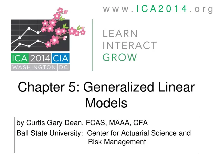
w w w . I C A 2 0 1 4 . o r g Chapter 5: Generalized Linear Models by Curtis Gary Dean, FCAS, MAAA, CFA Ball State University: Center for Actuarial Science and Risk Management

My Interest in Predictive Modeling  1989 article in Science  “Clinical Versus Actuarial Judgment”  Summarized in 1990 in Contingencies 2

“Clinical Versus Actuarial Judgment”  “In the clinical method the decision -maker combines or processes information in his or her head.”  “In the actuarial or statistical method the human judge is eliminated and conclusions rest solely on empirically established relations between data and the condition or event of interest.” 3

“Clinical Versus Actuarial Judgment”  “…with a sample of about 100 studies and the same outcome obtained in almost every case, it is reasonable to conclude that the actuarial advantage is not exceptional but general and likely encompasses many of the unstudied judgment tasks.” 4

“Clinical Versus Actuarial Judgment”  “To be truly actuarial, interpretations must be both automatic (that is, prespecified or routinized) and based on empirically established relations.”  Gary’s statement: “This is predictive modeling (predictive analytics).” 5

“Clinical Versus Actuarial Judgment”  “Even when given an information edge, the clinical judge still fails to surpass the actuarial method; in fact, access to additional information often does nothing to close the gap between the two methods.” 6

Why Use Generalized Linear Models?  Can readily see link between predictors and outcomes  Useful statistical tests for coefficients and fit of model  Easier to explain than some other methods  Software is widely available 7

Classical Multiple Linear Regression  μ i = E[ Y i ] = a 0 + a 1 X i 1 + …+ a m X im  Y i is Normally distributed random variable with constant variance σ 2  Want to estimate μ i = E[ Y i ] for each i 8

Response Y i has Normal Distribution μ i -12 -7 -2 3 8 9

Problems with Traditional Model  Number of claims is discrete  Claim sizes are skewed to the right  Probability of an event is in [0,1]  Variance is not constant across data points i  Nonlinear relationship between X ’s and Y ’s 10

Generalized Linear Models - GLMs  Fewer restrictions  Y can model number of claims, probability of renewing, loss severity, loss ratio, etc.  Large and small policies can be put into one model  Y can be nonlinear function of X’s  Classical linear regression model is a special case 11

Generalized Linear Models - GLMs  g ( μ i )= a 0 + a 1 X i 1 + …+ a m X im  g ( ) is the link function  E[ Y i ] = μ i = g -1 ( a 0 + a 1 X i 1 + …+ a m X im )  Y i can be Normal, Poisson, Gamma, Binomial, Compound Poisson, …  Variance can be modeled 12

Exponential Family of Distributions – Canonical Form             y b        f y ; , exp  c y ,       a   E [ Y ] b ' ( )    Var [ Y ] b ' ' ( ) a ( )  is the parameter of interest !  is often called a nuisance parameter. 13

Why Exponential Family?  Distributions in Exponential Family can model a variety of problems  Standard algorithm for finding coefficients a 0 , a 1 , …, a m 14

Normal Distribution in Exponential Family     2 1 ( y )       2 f ( y ; , ) exp    2    2 2 2           2 2 1 y 2 y         exp ln exp        2      2  2  2      2 2 y / 2 y       2 exp ln 2     2 2   2 15

Normal Distribution in Exponential Family θ b ( θ )      2 2 y / 2 y         2 2 f ( y ; , ) exp ln 2     2 2   2       2 Let and a ( ) ,           2 then b ( ) / 2 b ( )           2 2 and Var [ Y ] b ( ) a ( ) 1 16

Poisson Distribution in Exponential Family    y e   Pr[ Y y ] y !        y e       Pr[ Y y ] exp ln      y !  θ       (ln ) y      Pr[ Y y ] exp ln( y ! )   1 17

Compound Poisson Distribution  Y = C 1 + C 2 + . . . + C N  N is Poisson random variable  C i are i.i.d. with Gamma distribution  This is an example of a Tweedie distribution  Y is member of Exponential Family 18

Members of the Exponential Family • Normal • Poisson • Binomial • Gamma • Inverse Gaussian • Compound Poisson 19

Var[ Y i ] = Φ V( μ i )/ w i V ( μ )  0  Normal   Poisson  (1 -  )  Binomial  p , 1< p <2  Tweedie  2  Gamma  Inverse Gaussian  3 20

Variance of Y i and Fit at Data Point i  Var( Y i ) is big → looser fit at data point i  Var( Y i ) is small → tighter fit at data point i 1  Tightness of fit Var( Y ) i 21

Estimating Coefficients a 1 , a 2 , .., a m  Classical linear regression uses least squares  GLMs use Maximum Likelihood Method 22

Which Exponential Family Distribution?  Frequency: Poisson  Severity: Gamma  Loss ratio: Compound Poisson  Pure Premium: Compound Poisson  How many policies will renew: Binomial 23

What link function?  Additive model: identity  Multiplicative model: natural log  Modeling probability of event: logistic 24

Chapter 5: Generalized Linear Models  Intended as a first exposure to GLMs  Tried to make it accessible and self- contained  Hard to squeeze everything into one chapter – at Ball State the topic spans a semester-long course 25

5.1 Introduction to Generalized Linear Models 5.1.1 Assumptions of Linear Model - Shortcomings for actuarial applications 5.1.2 Generalized Linear Model Assumptions 26

5.2 Exponential Family of Distributions 5.2.1 The Variance Function and the Relationship between Variances and Means 5.3 Link Functions 5.4 Maximum Likelihood Estimation 5.2.1 Quasi-likelihood 5.5 Generalized Linear Model Review 27

5.6 Applications 5.6.1 Modeling Probability of Cross Selling with Logit Link 5.6.2 Claim Frequency with Offset 5.6.3 Severity with Weights 5.6.4 Modeling Pure Premiums or Loss Ratios 28

5.7 Comparing Models 5.7.1 Deviance 5.7.2 Log-likelihood, AIC, AICC, and BIC 29

The End 30