Chapter 3: Common Families of Distributions STK4011/9011: - PowerPoint PPT Presentation

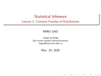
Chapter 3: Common Families of Distributions STK4011/9011: Statistical Inference Theory Johan Pensar STK4011/9011: Statistical Inference Theory Chapter 3: Common Families of Distributions 1 / 8

Overview Exponential Families 1 Location and Scale Families 2 Covers parts of Sec 3.4–3.5 in CB. STK4011/9011: Statistical Inference Theory Chapter 3: Common Families of Distributions 2 / 8

Families of Distributions Statistical distributions are used to model populations. We usually deal with a family of distributions, specified by one or more parameters. Discrete Distributions: the range of X is countable (often, integer-valued outcomes). Examples: Uniform, Hypergeometric, Binomial, Poisson, Geometric distribution (Sec 3.2). Continuous Distributions: the range of X is uncountable (e.g. interval on the real line). Examples: Uniform, Gamma, Normal, Beta, Cauchy, Lognormal distribution (Sec 3.3). STK4011/9011: Statistical Inference Theory Chapter 3: Common Families of Distributions 3 / 8

Exponential Families A family of pdfs or pmfs belong to the exponential family if it can be expressed as � k � � f ( x | θ ) = h ( x ) c ( θ ) exp w i ( θ ) t i ( x ) , i =1 where θ denotes the distribution parameter(s). h ( x ) ≥ 0 and t 1 ( x ) , . . . , t k ( x ) are real-valued functions of x , c ( θ ) ≥ 0 and w 1 ( θ ) , . . . , w k ( θ ) are real-valued functions of θ . The specific form of the above expression results in many nice properties (see e.g. Thm 3.4.2). STK4011/9011: Statistical Inference Theory Chapter 3: Common Families of Distributions 4 / 8

Example: Binomial exponential family STK4011/9011: Statistical Inference Theory Chapter 3: Common Families of Distributions 5 / 8

Location and Scale Families Thm 3.5.1: Let f ( x ) be any pdf and let µ and σ > 0 be any given constants. Then the function g ( x | µ, σ ) = 1 � x − µ � σ f σ is a pdf. STK4011/9011: Statistical Inference Theory Chapter 3: Common Families of Distributions 6 / 8

Location and Scale Families The family of pdfs g ( x | µ, σ ) is called the location-scale family, where f ( x ) = g ( x | µ = 0 , σ = 1) is called the standard pdf, µ is called the location parameter and shifts the location of the pdf (without modifying the shape), σ is called the scale parameter and adjusts the shape of pdf by stretching ( σ > 1) or contracting ( σ < 1). STK4011/9011: Statistical Inference Theory Chapter 3: Common Families of Distributions 7 / 8

Example: Normal distribution The (general) normal distribution e − ( x − µ )2 1 f ( x | µ, σ 2 ) = √ 2 σ 2 , −∞ < x < ∞ , 2 πσ is the location-scale family associated with the standard normal distribution. µ = 0 and σ = 1 µ = 1 and σ = 1 µ = 1 and σ = 0.5 µ = 1 and σ = 2 0.6 0.6 0.6 0.6 0.4 0.4 0.4 0.4 0.2 0.2 0.2 0.2 0.0 0.0 0.0 0.0 −6 −4 −2 0 2 4 6 −6 −4 −2 0 2 4 6 −6 −4 −2 0 2 4 6 −6 −4 −2 0 2 4 6 STK4011/9011: Statistical Inference Theory Chapter 3: Common Families of Distributions 8 / 8