Chapter 13 Quantifying Uncertainty CS5811 - Artificial Intelligence - PowerPoint PPT Presentation
Chapter 13 Quantifying Uncertainty CS5811 - Artificial Intelligence Nilufer Onder Department of Computer Science Michigan Technological University Outline Probability basics Syntax and semantics Inference Independence and Bayes rule
Chapter 13 Quantifying Uncertainty CS5811 - Artificial Intelligence Nilufer Onder Department of Computer Science Michigan Technological University
Outline Probability basics Syntax and semantics Inference Independence and Bayes’ rule
Motivation Uncertainty is everywhere. Consider the following proposition. A t : Leaving t minutes before the flight will get me to the airport. Problems: 1. partial observability (road state, other drivers’ plans, etc.) 2. noisy sensors (traffic reports, etc.) 3. uncertainty in action outcomes (flat tire, etc.) 4. immense complexity of modelling and predicting traffic
Knowledge representation Language Main elements Assignments Propositional logic facts T, F, unknown First-order logic facts, objects, relations T, F, unknown Temporal logic facts, objects, relations, times T, F, unknown Temporal CSPs time points time intervals Fuzzy logic set membership degree of truth Probability theory facts degree of belief The first three do not represent uncertainty, while the last three do.
Probability Probabilistic assertions summarize effects of laziness: failure to enumerate exceptions, qualifications, etc. ignorance: lack of relevant facts, initial conditions, etc. Probabilities relate propositions to one’s own state of knowledge. They might be learned from past experience of similar situations. e.g., P ( A 25 ) = 0.05 Probabilities of propositions change with new evidence: e.g., P ( A 25 | no reported accidents) = 0.06 e.g., P ( A 25 | no reported accidents, 5am) = 0.15
Probability basics Begin with a set Ω called the sample space A sample space is a set of possible outcomes Each ω ∈ Ω is a sample point ( possible world , atomic event ) e.g., 6 possible rolls of a die: { 1 , 2 , 3 , 4 , 5 , 6 } Probability space or probability model : Take a sample space Ω, and assign a number P( ω ) (the probability of ω ) to every atomic event ω ∈ Ω
Probability basics (cont’d) A probability space must satisfy the following properties: 0 ≤ P ( ω ) ≤ 1 for every ω ∈ Ω � ω ∈ Ω P ( ω ) = 1 e.g., for rolling the die, P (1) = P (2) = P (3) = P (4) = P (5) = P (6) = 1/6. An event A is any subset of Ω The probability of an event is defined as follows: P ( A ) = � { ω ∈ A } P ( ω ) e.g., P(die roll < 4) = P(1) + P(2) + P(3) = 1/6 + 1/6 + 1/6 = 1/2
Random variables A random variable is a function from sample points to some range such as integers or Booleans. We’ll use capitalized words for random variables. e.g., rolling the die: � true if ω is odd , Odd ( ω ) = false otherwise A probability distribution gives a probability for every possible value. If X is a random variable, then P ( X = x i ) = � { P ( ω ) : X ( ω ) = x i } e.g., P (Odd = true) = P (1) + P (3) + P (5) = 1/6 + 1/6 + 1/6 = 1/2 Note that we don’t write Odd’s argument ω here.
Propositions Odd is a Boolean or propositional random variable: its range is { true, false } We’ll use the corresponding lower-case word (in this case odd ) for the event that a propositional random variable is true e.g., P ( odd ) = P ( Odd = true ) = 3 / 6 P ( ¬ odd ) = P ( Odd = false ) = 3 / 6 Boolean formula = disjunction of the sample points in which it is true e.g., ( a ∨ b ) ≡ ( ¬ a ∧ b ) ∨ ( a ∧ ¬ b ) ∨ ( a ∧ b ) ⇒ P ( a ∨ b ) = P ( ¬ a ∧ b ) + P ( a ∧ ¬ b ) + P ( a ∧ b )
Syntax for propositions Propositional or Boolean random variables e.g., Cavity (do I have a cavity in one of my teeth?) Cavity = true is a proposition, also written cavity Discrete random variables (finite or infinite) e.g., Weather is one of < sunny , rain , cloudy , snow > Weather = rain is a proposition Values must be exhaustive and mutually exclusive Continuous random variables (bounded or unbounded) e.g., Temp = 21 . 6; Temp < 22 . 0 Arbitrary Boolean combinations of basic propositions e.g., ¬ cavity means Cavity = false Probabilities of propositions e.g., P ( cavity ) = 0.1 and P ( Weather = sunny ) = 0.72
Syntax for probability distributions Represent a discrete probability distribution as a vector of probability values: P ( Weather ) = < 0 . 72 , 0 . 1 , 0 . 08 , 0 . 1 > The above is an ordered list representing the probabilities of sunny , rain , cloudy , and snow . Probabilities of sunny , rain , cloudy , and snow must sum to 1 when the vector is normalized If B is a Boolean random variable, then P ( B ) = < P ( b ) , P ( ¬ b ) > e.g., if P ( cavity ) = 0 . 1 then P ( Cavity = true ) = 0 . 1 and P ( Cavity ) = < 0 . 1 , 0 . 9 > When the entries in the vector do not add up to 1, but represent the true ratios, the vector is preceded by a normalizing constant , α , e.g. P ( Cavity ) = α < 0 . 01 , 0 . 09 > where α is 10
Syntax for joint probability distributions A joint probability distribution for a set of n random variables gives the probability of every atomic event on those variables, i.e., every sample point Represent it as an n -dimensional matrix, e.g., P ( Weather , Cavity ) is a 4 × 2 matrix. The entries contain propabilities for all possible combinations of Weather (4), and Cavity (2). Weather = sunny rain cloudy snow Cavity = true 0.144 0.02 0.016 0.02 Cavity = false 0.576 0.08 0.064 0.08 Every question about a domain can be answered by the joint distribution because every event is a sum of sample points
Conditional probability Prior (unconditional) probabilities refer to degrees of belief in the absence of any other information. Posterior (conditional) probabilites refer to degrees of belief when we have some information, called evidence . Consider drawing straws from a set of 1 long and 4 short straws, long refers to drawing a long straw, and short refers to drawing a short straw. P ( long ) = 0.2 P ( long | short ) = 0.25 P ( long | long ) = 0.0 P ( long | short , short ) = 1 3 P ( long | rain ) = 0 . 2
Conditional probability (cont’d) P ( cavity | toothache ) = 0.8 means the probability of cavity given that toothache is all we know It does not mean “if toothache then 80% chance of cavity Suppose we get more evidence, e.g., cavity is also given. Then P ( cavity | toothache , cavity ) = 1 Note: the less specific belief remains valid, but is not always useful New evidence may be irrelevant, allowing simplification, e.g., P ( cavity | toothache , 49 ersWin ) = P ( cavity | toothache ) =0.8 Conditional distibutions are shown as vectors for all possible combinations of the evidence and query. P ( Cavity | Toothache ) is a 2-element vector of 2-element vectors < < 0 . 12 , 0 . 08 > , < 0 . 08 , 0 . 72 > > � �� � � �� � toothache ¬ toothache
Conditional probability definitions Definition of conditional probability: P ( a | b ) = P ( a ∧ b ) P ( b ) Product rule gives an alternative formulation and holds even if P ( b ) = 0 P ( a ∧ b ) = P ( a | b ) P ( b ) = P ( b | a ) P ( a ) A general version holds for an entire probability distribution, e.g., P ( Weather , Cavity ) = P ( Weather | Cavity ) P ( Cavity ) This is not matrix multiplication, it’s a set of 4 × 2 equations: P ( sunny , cavity ) = P ( sunny | cavity ) P ( cavity ) P ( sunny , ¬ cavity ) = P ( sunny |¬ cavity ) P ( ¬ cavity ) P ( rain , cavity ) = P ( rain | cavity ) P ( cavity ) P ( rain , ¬ cavity ) = P ( rain |¬ cavity ) P ( ¬ cavity ) P ( cloudy , cavity ) = P ( cloudy | cavity ) P ( cavity ) P ( cloudy , ¬ cavity ) = P ( cloudy |¬ cavity ) P ( ¬ cavity ) P ( snow , cavity ) = P ( snow | cavity ) P ( cavity ) P ( snow , ¬ cavity ) = P ( snow |¬ cavity ) P ( ¬ cavity )
Chain rule Chain rule is derived by successive applications of the product rule: P ( X 1 , . . . , X n ) = P ( X n | X 1 , . . . , X n − 1 ) P ( X 1 , . . . , X n − 1 ) = P ( X n | X 1 , . . . , X n − 1 ) P ( X n − 1 | X 1 , . . . , X n − 2 ) P ( X 1 , . . . , X n − 2 ) = . . . = � n i =1 P ( X i | X 1 , . . . , X i − 1 ) For example, P ( X 1 , X 2 , X 3 , X 4 ) = P ( X 1 ) P ( X 2 | X 1 ) P ( X 3 | X 1 , X 2 ) P ( X 4 | X 1 , X 2 , X 3 ) = P ( X 4 | X 3 , X 2 , X 1 ) P ( X 3 | X 2 , X 1 ) P ( X 2 | X 1 ) P ( X 1 )
Inference by enumeration The Dentist Domain : What is the probability of a cavity given a toothache ? What is the probability of a cavity given the probe catch es? We start with the joint distribution: toothache ~toothache catch ~catch catch ~catch cavity .108 .012 .072 .008 ~cavity .016 .064 .144 .576 For any proposition q , add up the atomic events where it is true: � P ( q ) = P ( w ) w : w | = q
Computing the probability of a proposition toothache ~toothache catch ~catch catch ~catch cavity .108 .012 .072 .008 ~cavity .016 .064 .144 .576 For any proposition q , add up the atomic events where it is true: � P ( q ) = P ( w ) w : w | = q Red shows “the world” given what we know so far. Green shows the (atomic) event we are interested in. P ( toothache )= P ( toothache , catch , cavity ) + P ( toothache , ¬ catch , cavity )+ P ( toothache , catch , ¬ cavity ) + P ( toothache , ¬ catch , ¬ cavity ) = 0.108 + 0.012 + 0.016 + 0.064 = 0.2
Computing the probability of a logical sentence toothache ~toothache catch ~catch catch ~catch cavity .108 .012 .072 .008 ~cavity .016 .064 .144 .576 P ( cavity ∨ toothache ) = 0.108 + 0.012 + 0.072 + 0.008 + 0.016 + 0.064 = 0.28
Recommend
More recommend
Explore More Topics
Stay informed with curated content and fresh updates.
