Challenges and Techniques for Efficient Contour Covering using - PowerPoint PPT Presentation
Challenges and Techniques for Efficient Contour Covering using Collaborating Mobile Sensors Sumana Srinivasan Advisor : Dr. Krithi Ramamritham Co-advisor : Dr. Purushottam Kulkarni Department of Computer Science and Engineering Indian Institute
Challenges and Techniques for Efficient Contour Covering using Collaborating Mobile Sensors Sumana Srinivasan Advisor : Dr. Krithi Ramamritham Co-advisor : Dr. Purushottam Kulkarni Department of Computer Science and Engineering Indian Institute of Technology Bombay, Mumbai, INDIA Pre-synopsis Seminar, March 26th, 2010 1 / 94
A spill and its “wake”(up call)!! F IG . 2: Statfjord spill, 2007 F IG . 1: Exxon spill, 1989 — Millions of marine life forms destroyed. ◮ Inefficient way of determining extent and mitigating spread!! ◮ Could the unprecedented adverse impact of this disaster been diminished by a quicker and more efficient response? 2 / 94
Cyber Physical Systems to the rescue!! F IG . 3: Applications of CPS Can advances in CPS be used to determine extent and mitigation of disasters? F IG . 4: Applications of CPS 3 / 94
Challenges for CPS ◮ Can CPS determine the exact location and extent of the most hazardous region accurately? ◮ Can the region be covered energy efficiently to contain the spill and perform remedial actions making best use of information that is available? ◮ Can the system achieve best coverage under energy constraints ? ◮ Can they adapt to limitations of the system such as — limited sensing, communication range and energy available? 4 / 94
How do you determine extent? Contour estimation — determining extent of “hazardous region” and sources of contamination. Parameters ◮ Temperature ◮ Pressure ◮ Depth ◮ Light intensity ◮ Concentration ◮ Salinity ◮ Density F IG . 5: A light field with light intensity contours. ◮ A contour is defined as a set of points of equal value of a specified parameter. 5 / 94
Outline ◮ Motivation ◮ Challenges and Contributions ◮ System model, Problem formulation and Evaluation metrics ◮ Evolution of strategies based on Information Utilization ◮ Our Solution — Ingredients and evaluation ◮ Conclusions 6 / 94
Existing techniques for contour estimation Techniques Accuracy Minimize Physically Perform Adaptive depends cover the remedial to spatio- upon contour actions temporal dynamics Remote Image Error No No Yes sensing Resolution Static High Communication No No No sensor node cost networks density Mobile Number of Movement Yes Yes Yes sensor samples cost networks 7 / 94
Mobile sensors - State of the art ◮ SOTAB1 — image sensors, viscosity sensors, wind and depth meter, water thermometers. ◮ Dorado - Used for mapping the sea bed equipped with sonars. ◮ Robotic carp — tiny chemical sensors in the port of Gijon in northern Spain to find sources of pollutants in the water. Energy consumption due to movement — COSTLY!!! 8 / 94
Contour Covering Problem CCP Using a network of mobile sensors, can we determine the location and extent of a hazardous contour in a bounded sensing region and cover it accurately in an energy efficient manner? Objectives ◮ Maximize the coverage of contour ⇒ hazardous region of the spill is contained. ◮ Minimize the coverage of nonrelevant regions ⇒ better resource utilization. ◮ Minimize energy consumption due to movement and response time ⇒ increase lifetime and timely action. 9 / 94
System Model and Assumptions 2D Model Notations. Assumptions ◮ Target contour continuous and static w.r.t. sensors. ◮ Sensors are location aware. ◮ No odometry errors. ◮ Sensing measurements are smoothened by averaging. 10 / 94
Fundamental Challenges of CCP 1. Which direction should the sensor move ? ◮ How does the sensor make a nontrivial decision of choosing one direction over others given the constraints of the system? ◮ What factors does this decision depend upon? ◮ Are there any trade-offs in choosing one direction over any other? 2. What information is needed to determine direction? How is the information gathered and utilized? 11 / 94
Contributions 1. A novel formulation to the Contour Covering Problem (CCP) with maximizing coverage, minimizing coverage error and energy consumption. 2. A proof of hardness for the optimal latency for CCP . 3. Motion planning algorithms based on information exploitation ◮ Baseline:Gradient Descent G and Surround S ◮ Minimizing Centroid Distance MCD [Srinivasan and Ramamritham, 2006] ◮ Centralized Periodic Udate Adaptive Contour Estimation ACE [S.Srinivasan et al., 2008] ◮ Energy-aware Distributed and Adaptive Contour Covering E 4. Extensive performance evaluation of the algorithms ◮ deployments, contours, energy constraints, number of sensors, communication range and sensing error. 5. Comparison with optimal latency and previous mobility strategies.. 12 / 94
Evaluation Metrics Coverage. C and Coverage Error, ℵ C = Area of ( C est ∩ C act ) Area of C act ℵ = Area of ([ C reg − C act ] ∩ C est ) Area of [ C reg − C act ] Latency, L L = max ( T 1 , T 2 , . . . , T m ) (1) Precision, φ and F-measures, F β Φ = Area of ( C est ∩ C act ) Area of C est F β = ( 1 + β 2 ) × Φ × C β 2 × Φ + C GO 13 / 94
Contour Covering Problem CCP Definition Given N mobile sensors s 1 , · · · s N , ◮ each with energy, e init i ◮ deployed in a 2D bounded sensing region R ≡ [ l × l ] , ◮ defined by a scalar field f such that f ( x , y ) ∈ [ L , U ] (where L and U are lower and upper bounds of the field value) and ◮ value of the target contour τ ∈ [ L , U ] , the goal is to determine the points on the estimated level set in order to 1. Maximize coverage, C subjected to constraints, 1. Minimize coverage error, ℵ 2. Minimize latency, L 14 / 94
Movement Phases and Termination Condition Movement Phases ◮ Converge Phase : Movement towards the contour until the sensor hits the contour ◮ Coverage Phase : Movement along the contour until termination. Termination Conditions ◮ Condition I : When none of the sensors have energy to move. ◮ Condition II : When the contour is fully estimated or every point on the contour is visited by at least one sensor (i.e., C = 100 % and ℵ = 0 % ). 15 / 94
Type of Information 16 / 94
Strategies for CCP based on information utilization Strategy 1 — Complete Information ◮ Information: Locations of contour points and locations of other sensors are known to a sensor ◮ Technique: Determination of optimal latency for CCP (OPTCCP) is NP Complete. MTSP reduces to OPTCCP . Strategy 2 — No information ◮ Information: Measurement at current location only known to a sensor ◮ Techniques: 1. Exhaustive search, based on space filling curves [Spires and Goldsmith, 1998] to locate the contour — worst case O ( l 2 ) 2. Random search, based on random walk to locate the contour — worst case O (( l 2 ) 3 ) (Brightwell Winkler Theorem [G. and P ., 1990]) 17 / 94
Strategies for CCP , contd. Strategy 3 — Overlap information ◮ Information: Location and field values from other sensors are known to a sensor and overlap w.r.t. contour. ◮ Techniques: 1. All sensors inside, move in the direction of maximizing hull area. 2. All sensors outside and overlapping, move in the direction of minimizing hull area, 3. If no overlap, how should they determine the direction of movement? 18 / 94
Strategies for CCP , contd. Strategy 4 — Gradient information ∇ f = ( ∂ f ∂ x , ∂ f ∂ y ) ∂ f ∂ x = f ( x + h ) − f ( x ) h ◮ Information: Location and field value from all sensors. ◮ Techniques: 1. Clustered deployments to minimize h , spatially correlated readings to determine ∇ f [Marthaler and Bertozzi, 2004, Zhang and Leonard, 2005]. 2. Use exporation to determine samples for approximating gradient. 3. Can sensors that can sense beyond their location be used? 19 / 94
Are measurable gradients present within r s ? Sensors r s Concentration/Slick Thickness Height Laser fluorosensor up to 50m submicrons 3m SlickSleuth several meters 0.001% 1.5 - 5m ◮ Take home: If deployed close to the spill (within 100kms) quickly (within 0.5d), steep gradients (0-60ppb) can be found within a spatial resolution of 1m which can be detected by sensors today. OIL MODEL 20 / 94
Gradient Descent Algorithm, G Information Uses only measurements within r s to determine direction of approach. Technique Define artificial potential gradient function , � ( 1 − f ( x , y ) ) 2 if f ( x , y ) ≤ τ g f ( x , y ) = τ (2) f ( x , y ) ) 2 τ ( 1 − if f ( x , y ) > τ ◮ G moves in the direction that minimizes g f or moves in the direction of steepest gradient. ◮ If f is a continuous convex function, then g f is convex with a minimum at f = τ . ◮ Perform exploration in the absence of gradients (spiral search) 21 / 94
Limitations of G ◮ When sensors are clustered — does not maximize coverage under energy constraints ◮ Higher latency in the absence of energy constraints. ◮ Sensors can get into local F IG . 6: Gradient minima in a non-uniform field. descent under clustered deployment Can sensors move in a direction that approaches as well as spread out with respect to contour? 22 / 94
Surrounding the contour Information ◮ Inputs are centroid of the contour, measurements within r s and location information from other sensors. Technique Angular distribution around centroid. ◮ Compute and assign target angles such that the total angular difference is minimized, the Hungarian algorithm [H.W.Kuhn, 1955]. 23 / 94
Recommend


More recommend
Explore More Topics
Stay informed with curated content and fresh updates.